On-Device Training with LiteRT

Licensed under the Apache License, Version 2.0 (the "License");

  # 
  
 you 
  
 may 
  
 not 
  
 use 
  
 this 
  
 file 
  
 except 
  
 in 
  
 compliance 
  
 with 
  
 the 
  
 License 
 . 
 # 
  
 You 
  
 may 
  
 obtain 
  
 a 
  
 copy 
  
 of 
  
 the 
  
 License 
  
 at 
 # 
 # 
  
 https 
 : 
 //www.apache.org/licenses/LICENSE-2.0 
 # 
 # 
  
 Unless 
  
 required 
  
 by 
  
 applicable 
  
 law 
  
 or 
  
 agreed 
  
 to 
  
 in 
  
 writing 
 , 
  
 software 
 # 
  
 distributed 
  
 under 
  
 the 
  
 License 
  
 is 
  
 distributed 
  
 on 
  
 an 
  
 "AS IS" 
  
 BASIS 
 , 
 # 
  
 WITHOUT 
  
 WARRANTIES 
  
 OR 
  
 CONDITIONS 
  
 OF 
  
 ANY 
  
 KIND 
 , 
  
 either 
  
 express 
  
 or 
  
 implied 
 . 
 # 
  
 See 
  
 the 
  
 License 
  
 for 
  
 the 
  
 specific 
  
 language 
  
 governing 
  
 permissions 
  
 and 
 # 
  
 limitations 
  
 under 
  
 the 
  
 License 
 . 
 
Run in Google Colab View source on GitHub Download notebook

When deploying LiteRT machine learning model to device or mobile app, you may want to enable the model to be improved or personalized based on input from the device or end user. Using on-device training techniques allows you to update a model without data leaving your users' devices, improving user privacy, and without requiring users to update the device software.

For example, you may have a model in your mobile app that recognizes fashion items, but you want users to get improved recognition performance over time based on their interests. Enabling on-device training allows users who are interested in shoes to get better at recognizing a particular style of shoe or shoe brand the more often they use your app.

This tutorial shows you how to construct a LiteRT model that can be incrementally trained and improved within an installed Android app.

Setup

This tutorial uses Python to train and convert a TensorFlow model before incorporating it into an Android app. Get started by installing and importing the following packages.
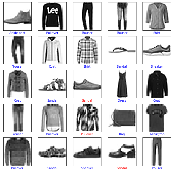
  import 
  
 matplotlib.pyplot 
  
 as 
  
 plt 
 import 
  
 numpy 
  
 as 
  
 np 
 import 
  
 tensorflow 
  
 as 
  
 tf 
 print 
 ( 
 "TensorFlow version:" 
 , 
 tf 
 . 
 __version__ 
 ) 
 
TensorFlow version: 2.8.0

Classify images of clothing

This example code uses the Fashion MNIST dataset to train a neural network model for classifying images of clothing. This dataset contains 60,000 small (28 x 28 pixel) grayscale images containing 10 different categories of fashion accessories, including dresses, shirts, and sandals.

Fashion MNIST images
Figure 1 : Fashion-MNIST samples (by Zalando, MIT License).

You can explore this dataset in more depth in the Keras classification tutorial .

Build a model for on-device training

LiteRT models typically have only a single exposed function method (or signature ) that allows you to call the model to run an inference. For a model to be trained and used on a device, you must be able to perform several separate operations, including train, infer, save, and restore functions for the model. You can enable this functionality by first extending your TensorFlow model to have multiple functions, and then exposing those functions as signatures when you convert your model to the LiteRT model format.

The code example below shows you how to add the following functions to a TensorFlow model:

  • train function trains the model with training data.
  • infer function invokes the inference.
  • save function saves the trainable weights into the file system.
  • restore function loads the trainable weights from the file system.
  IMG_SIZE 
  
 = 
  
 28 
 class 
  
 Model 
 ( 
 tf 
 . 
 Module 
 ) 
 : 
  
 def 
  
 __init__ 
 ( 
 self 
 ) 
 : 
  
 self 
 . 
 model 
  
 = 
  
 tf 
 . 
 keras 
 . 
 Sequential 
 ( 
 [ 
  
 tf 
 . 
 keras 
 . 
 layers 
 . 
 Flatten 
 ( 
 input_shape 
 = 
 ( 
 IMG_SIZE 
 , 
  
 IMG_SIZE 
 ), 
  
 name 
 = 
 'flatten' 
 ), 
  
 tf 
 . 
 keras 
 . 
 layers 
 . 
 Dense 
 ( 
 128 
 , 
  
 activation 
 = 
 'relu' 
 , 
  
 name 
 = 
 'dense_1' 
 ), 
  
 tf 
 . 
 keras 
 . 
 layers 
 . 
 Dense 
 ( 
 10 
 , 
  
 name 
 = 
 'dense_2' 
 ) 
  
 ] 
 ) 
  
 self 
 . 
 model 
 . 
 compile 
 ( 
  
 optimizer 
 = 
 'sgd' 
 , 
  
 loss 
 = 
 tf 
 . 
 keras 
 . 
 losses 
 . 
 CategoricalCrossentropy 
 ( 
 from_logits 
 = 
 True 
 )) 
  
 # The `train` function takes a batch of input images and labels. 
  
 @tf.function 
 ( 
 input_signature 
 = 
 [ 
  
 tf 
 . 
 TensorSpec 
 ( 
 [ 
 None 
 , 
  
 IMG_SIZE 
 , 
  
 IMG_SIZE 
 ] 
 , 
  
 tf 
 . 
 float32 
 ), 
  
 tf 
 . 
 TensorSpec 
 ( 
 [ 
 None 
 , 
  
 10 
 ] 
 , 
  
 tf 
 . 
 float32 
 ), 
  
 ] 
 ) 
  
 def 
  
 train 
 ( 
 self 
 , 
  
 x 
 , 
  
 y 
 ) 
 : 
  
 with 
  
 tf 
 . 
 GradientTape 
 () 
  
 as 
  
 tape 
 : 
  
 prediction 
  
 = 
  
 self 
 . 
 model 
 ( 
 x 
 ) 
  
 loss 
  
 = 
  
 self 
 . 
 model 
 . 
 loss 
 ( 
 y 
 , 
  
 prediction 
 ) 
  
 gradients 
  
 = 
  
 tape 
 . 
 gradient 
 ( 
 loss 
 , 
  
 self 
 . 
 model 
 . 
 trainable_variables 
 ) 
  
 self 
 . 
 model 
 . 
 optimizer 
 . 
 apply_gradients 
 ( 
  
 zip 
 ( 
 gradients 
 , 
  
 self 
 . 
 model 
 . 
 trainable_variables 
 )) 
  
 result 
  
 = 
  
 { 
 "loss" 
 : 
  
 loss 
 } 
  
 return 
  
 result 
  
 @tf.function 
 ( 
 input_signature 
 = 
 [ 
  
 tf 
 . 
 TensorSpec 
 ( 
 [ 
 None 
 , 
  
 IMG_SIZE 
 , 
  
 IMG_SIZE 
 ] 
 , 
  
 tf 
 . 
 float32 
 ), 
  
 ] 
 ) 
  
 def 
  
 infer 
 ( 
 self 
 , 
  
 x 
 ) 
 : 
  
 logits 
  
 = 
  
 self 
 . 
 model 
 ( 
 x 
 ) 
  
 probabilities 
  
 = 
  
 tf 
 . 
 nn 
 . 
 softmax 
 ( 
 logits 
 , 
  
 axis 
 =- 
 1 
 ) 
  
 return 
  
 { 
  
 "output" 
 : 
  
 probabilities 
 , 
  
 "logits" 
 : 
  
 logits 
  
 } 
  
 @tf.function 
 ( 
 input_signature 
 = 
 [ 
 tf 
 . 
 TensorSpec 
 ( 
 shape 
 = 
 [] 
 , 
  
 dtype 
 = 
 tf 
 . 
 string 
 ) 
 ] 
 ) 
  
 def 
  
 save 
 ( 
 self 
 , 
  
 checkpoint_path 
 ) 
 : 
  
 tensor_names 
  
 = 
  
 [ 
 weight 
 . 
 name 
  
 for 
  
 weight 
  
 in 
  
 self 
 . 
 model 
 . 
 weights 
 ] 
  
 tensors_to_save 
  
 = 
  
 [ 
 weight 
 . 
 read_value 
 () 
  
 for 
  
 weight 
  
 in 
  
 self 
 . 
 model 
 . 
 weights 
 ] 
  
 tf 
 . 
 raw_ops 
 . 
 Save 
 ( 
  
 filename 
 = 
 checkpoint_path 
 , 
  
 tensor_names 
 = 
 tensor_names 
 , 
  
 data 
 = 
 tensors_to_save 
 , 
  
 name 
 = 
 'save' 
 ) 
  
 return 
  
 { 
  
 "checkpoint_path" 
 : 
  
 checkpoint_path 
  
 } 
  
 @tf.function 
 ( 
 input_signature 
 = 
 [ 
 tf 
 . 
 TensorSpec 
 ( 
 shape 
 = 
 [] 
 , 
  
 dtype 
 = 
 tf 
 . 
 string 
 ) 
 ] 
 ) 
  
 def 
  
 restore 
 ( 
 self 
 , 
  
 checkpoint_path 
 ) 
 : 
  
 restored_tensors 
  
 = 
  
 {} 
  
 for 
  
 var 
  
 in 
  
 self 
 . 
 model 
 . 
 weights 
 : 
  
 restored 
  
 = 
  
 tf 
 . 
 raw_ops 
 . 
 Restore 
 ( 
  
 file_pattern 
 = 
 checkpoint_path 
 , 
  
 tensor_name 
 = 
 var 
 . 
 name 
 , 
  
 dt 
 = 
 var 
 . 
 dtype 
 , 
  
 name 
 = 
 'restore' 
 ) 
  
 var 
 . 
 assign 
 ( 
 restored 
 ) 
  
 restored_tensors 
 [ 
 var 
 . 
 name 
 ] 
  
 = 
  
 restored 
  
 return 
  
 restored_tensors 
 

The train function in the code above uses the GradientTape class to record operations for automatic differentiation. For more information on how to use this class, see the Introduction to gradients and automatic differentiation .

You could use the Model.train_step method of the keras model here instead of a from-scratch implementation. Just note that the loss (and metrics) returned by Model.train_step is the running average, and should be reset regularly (typically each epoch). See Customize Model.fit for details.

Prepare the data

Get the Fashion MNIST dataset for training your model.

  fashion_mnist 
  
 = 
  
 tf 
 . 
 keras 
 . 
 datasets 
 . 
 fashion_mnist 
 ( 
 train_images 
 , 
  
 train_labels 
 ), 
  
 ( 
 test_images 
 , 
  
 test_labels 
 ) 
  
 = 
  
 fashion_mnist 
 . 
 load_data 
 () 
 

Preprocess the dataset

Pixel values in this dataset are between 0 and 255, and must be normalized to a value between 0 and 1 for processing by the model. Divide the values by 255 to make this adjustment.

  train_images 
  
 = 
  
 ( 
 train_images 
  
 / 
  
 255.0 
 ). 
 astype 
 ( 
 np 
 . 
 float32 
 ) 
 test_images 
  
 = 
  
 ( 
 test_images 
  
 / 
  
 255.0 
 ). 
 astype 
 ( 
 np 
 . 
 float32 
 ) 
 

Convert the data labels to categorical values by performing one-hot encoding.

 train_labels = tf.keras.utils.to_categorical(train_labels)
test_labels = tf.keras.utils.to_categorical(test_labels) 

Train the model

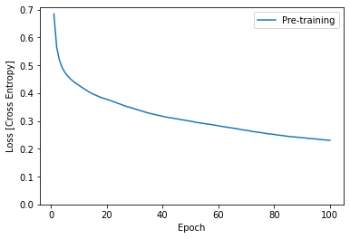
Before converting and setting up your LiteRT model, complete the initial training of your model using the preprocessed dataset and the train signature method. The following code runs model training for 100 epochs, processing batches of 100 images at a time, and displaying the loss value after every 10 epochs. Since this training run is processing quite a bit of data, it may take a few minutes to finish.

  NUM_EPOCHS 
  
 = 
  
 100 
 BATCH_SIZE 
  
 = 
  
 100 
 epochs 
  
 = 
  
 np 
 . 
 arange 
 ( 
 1 
 , 
  
 NUM_EPOCHS 
  
 + 
  
 1 
 , 
  
 1 
 ) 
 losses 
  
 = 
  
 np 
 . 
 zeros 
 ( 
 [ 
 NUM_EPOCHS 
 ] 
 ) 
 m 
  
 = 
  
 Model 
 () 
 train_ds 
  
 = 
  
 tf 
 . 
 data 
 . 
 Dataset 
 . 
 from_tensor_slices 
 (( 
 train_images 
 , 
  
 train_labels 
 )) 
 train_ds 
  
 = 
  
 train_ds 
 . 
 batch 
 ( 
 BATCH_SIZE 
 ) 
 for 
  
 i 
  
 in 
  
 range 
 ( 
 NUM_EPOCHS 
 ) 
 : 
  
 for 
  
 x 
 , 
 y 
  
 in 
  
 train_ds 
 : 
  
 result 
  
 = 
  
 m 
 . 
 train 
 ( 
 x 
 , 
  
 y 
 ) 
  
 losses 
 [ 
 i 
 ] 
  
 = 
  
 result 
 [ 
 'loss' 
 ] 
  
 if 
  
 ( 
 i 
  
 + 
  
 1 
 ) 
  
 % 
  
 10 
  
 == 
  
 0 
 : 
  
 print 
 ( 
 f 
 "Finished {i+1} epochs" 
 ) 
  
 print 
 ( 
 f 
 "  loss: {losses[i]:.3f}" 
 ) 
 # 
  
 Save 
  
 the 
  
 trained 
  
 weights 
  
 to 
  
 a 
  
 checkpoint 
 . 
 m 
 . 
 save 
 ( 
 '/tmp/model.ckpt' 
 ) 
 
Finished 10 epochs
  loss: 0.428
Finished 20 epochs
  loss: 0.378
Finished 30 epochs
  loss: 0.344
Finished 40 epochs
  loss: 0.317
Finished 50 epochs
  loss: 0.299
Finished 60 epochs
  loss: 0.283
Finished 70 epochs
  loss: 0.266
Finished 80 epochs
  loss: 0.252
Finished 90 epochs
  loss: 0.240
Finished 100 epochs
  loss: 0.230
{'checkpoint_path'&colon; <tf.Tensor&colon; shape=(), dtype=string, numpy=b'/tmp/model.ckpt'>}
  plt 
 . 
 plot 
 ( 
 epochs 
 , 
  
 losses 
 , 
  
 label 
 = 
 ' 
 Pre 
 - 
 training 
 ' 
 ) 
 plt 
 . 
 ylim 
 ([ 
 0 
 , 
  
 max 
 ( 
 plt 
 . 
 ylim 
 ())]) 
 plt 
 . 
 xlabel 
 ( 
 ' 
 Epoch 
 ' 
 ) 
 plt 
 . 
 ylabel 
 ( 
 ' 
 Loss 
  
 [ 
 Cross 
  
 Entropy 
 ] 
 ' 
 ) 
 plt 
 . 
 legend 
 (); 
 

png

Convert model to LiteRT format

After you have extended your TensorFlow model to enable additional functions for on-device training and completed initial training of the model, you can convert it to LiteRT format. The following code converts and saves your model to that format, including the set of signatures that you use with the LiteRT model on a device: train, infer, save, restore .

  SAVED_MODEL_DIR 
  
 = 
  
 "saved_model" 
 tf 
 . 
 saved_model 
 . 
 save 
 ( 
  
 m 
 , 
  
 SAVED_MODEL_DIR 
 , 
  
 signatures 
 = 
 { 
  
 'train' 
 : 
  
 m 
 . 
 train 
 . 
 get_concrete_function 
 (), 
  
 'infer' 
 : 
  
 m 
 . 
 infer 
 . 
 get_concrete_function 
 (), 
  
 'save' 
 : 
  
 m 
 . 
 save 
 . 
 get_concrete_function 
 (), 
  
 'restore' 
 : 
  
 m 
 . 
 restore 
 . 
 get_concrete_function 
 (), 
  
 }) 
 # Convert the model 
 converter 
  
 = 
  
 tf 
 . 
 lite 
 . 
 TFLiteConverter 
 . 
 from_saved_model 
 ( 
 SAVED_MODEL_DIR 
 ) 
 converter 
 . 
 target_spec 
 . 
 supported_ops 
  
 = 
  
 [ 
  
 tf 
 . 
 lite 
 . 
 OpsSet 
 . 
 TFLITE_BUILTINS 
 , 
  
 # enable LiteRT ops. 
  
 tf 
 . 
 lite 
 . 
 OpsSet 
 . 
 SELECT_TF_OPS 
  
 # enable TensorFlow ops. 
 ] 
 converter 
 . 
 experimental_enable_resource_variables 
  
 = 
  
 True 
 tflite_model 
  
 = 
  
 converter 
 . 
 convert 
 () 
 

Setup the LiteRT signatures

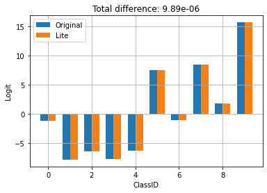
The LiteRT model you saved in the previous step contains several function signatures. You can access them through the tf.lite.Interpreter class and invoke each restore , train , save , and infer signature separately.

 interpreter = tf.lite.Interpreter(model_content=tflite_model)
interpreter.allocate_tensors()

infer = interpreter.get_signature_runner("infer") 

Compare the output of the original model, and the converted lite model:

 logits_original = m.infer(x=train_images[:1])['logits'][0]
logits_lite = infer(x=train_images[:1])['logits'][0] 

 def compare_logits(logits):
  width = 0.35
  offset = width/2
  assert len(logits)==2

  keys = list(logits.keys())
  plt.bar(x = np.arange(len(logits[keys[0]]))-offset,
      height=logits[keys[0]], width=0.35, label=keys[0])
  plt.bar(x = np.arange(len(logits[keys[1]]))+offset,
      height=logits[keys[1]], width=0.35, label=keys[1])
  plt.legend()
  plt.grid(True)
  plt.ylabel('Logit')
  plt.xlabel('ClassID')

  delta = np.sum(np.abs(logits[keys[0]] - logits[keys[1]]))
  plt.title(f"Total difference: {delta:.3g}")

compare_logits({'Original': logits_original, 'Lite': logits_lite}) 

png

Above, you can see that the behavior of the model is not changed by the conversion to TFLite.

Retrain the model on a device

After converting your model to LiteRT and deploying it with your app, you can retrain the model on a device using new data and the train signature method of your model. Each training run generates a new set of weights that you can save for re-use and further improvement of the model, as shown in the next section.

On Android, you can perform on-device training with LiteRT using either Java or C++ APIs. In Java, use the Interpreter class to load a model and drive model training tasks. The following example shows how to run the training procedure using the runSignature method:

  try 
  
 ( 
 Interpreter 
  
 interpreter 
  
 = 
  
 new 
  
 Interpreter 
 ( 
 modelBuffer 
 )) 
  
 { 
  
 int 
  
 NUM_EPOCHS 
  
 = 
  
 100 
 ; 
  
 int 
  
 BATCH_SIZE 
  
 = 
  
 100 
 ; 
  
 int 
  
 IMG_HEIGHT 
  
 = 
  
 28 
 ; 
  
 int 
  
 IMG_WIDTH 
  
 = 
  
 28 
 ; 
  
 int 
  
 NUM_TRAININGS 
  
 = 
  
 60000 
 ; 
  
 int 
  
 NUM_BATCHES 
  
 = 
  
 NUM_TRAININGS 
  
 / 
  
 BATCH_SIZE 
 ; 
  
 List<FloatBuffer> 
  
 trainImageBatches 
  
 = 
  
 new 
  
 ArrayList 
<> ( 
 NUM_BATCHES 
 ); 
  
 List<FloatBuffer> 
  
 trainLabelBatches 
  
 = 
  
 new 
  
 ArrayList 
<> ( 
 NUM_BATCHES 
 ); 
  
 // Prepare training batches. 
  
 for 
  
 ( 
 int 
  
 i 
  
 = 
  
 0 
 ; 
  
 i 
 < 
 NUM_BATCHES 
 ; 
  
 ++ 
 i 
 ) 
  
 { 
  
 FloatBuffer 
  
 trainImages 
  
 = 
  
 FloatBuffer 
 . 
 allocateDirect 
 ( 
 BATCH_SIZE 
  
 * 
  
 IMG_HEIGHT 
  
 * 
  
 IMG_WIDTH 
 ). 
 order 
 ( 
 ByteOrder 
 . 
 nativeOrder 
 ()); 
  
 FloatBuffer 
  
 trainLabels 
  
 = 
  
 FloatBuffer 
 . 
 allocateDirect 
 ( 
 BATCH_SIZE 
  
 * 
  
 10 
 ). 
 order 
 ( 
 ByteOrder 
 . 
 nativeOrder 
 ()); 
  
 // Fill the data values... 
  
 trainImageBatches 
 . 
 add 
 ( 
 trainImages 
 . 
 rewind 
 ()); 
  
 trainImageLabels 
 . 
 add 
 ( 
 trainLabels 
 . 
 rewind 
 ()); 
  
 } 
  
 // Run training for a few steps. 
  
 float 
 [] 
  
 losses 
  
 = 
  
 new 
  
 float 
 [ 
 NUM_EPOCHS 
 ] 
 ; 
  
 for 
  
 ( 
 int 
  
 epoch 
  
 = 
  
 0 
 ; 
  
 epoch 
 < 
 NUM_EPOCHS 
 ; 
  
 ++ 
 epoch 
 ) 
  
 { 
  
 for 
  
 ( 
 int 
  
 batchIdx 
  
 = 
  
 0 
 ; 
  
 batchIdx 
 < 
 NUM_BATCHES 
 ; 
  
 ++ 
 batchIdx 
 ) 
  
 { 
  
 Map<String 
 , 
  
 Object 
>  
 inputs 
  
 = 
  
 new 
  
 HashMap 
<> (); 
  
 inputs 
 . 
 put 
 ( 
 "x" 
 , 
  
 trainImageBatches 
 . 
 get 
 ( 
 batchIdx 
 )); 
  
 inputs 
 . 
 put 
 ( 
 "y" 
 , 
  
 trainLabelBatches 
 . 
 get 
 ( 
 batchIdx 
 )); 
  
 Map<String 
 , 
  
 Object 
>  
 outputs 
  
 = 
  
 new 
  
 HashMap 
<> (); 
  
 FloatBuffer 
  
 loss 
  
 = 
  
 FloatBuffer 
 . 
 allocate 
 ( 
 1 
 ); 
  
 outputs 
 . 
 put 
 ( 
 "loss" 
 , 
  
 loss 
 ); 
  
 interpreter 
 . 
 runSignature 
 ( 
 inputs 
 , 
  
 outputs 
 , 
  
 "train" 
 ); 
  
 // Record the last loss. 
  
 if 
  
 ( 
 batchIdx 
  
 == 
  
 NUM_BATCHES 
  
 - 
  
 1 
 ) 
  
 losses 
 [ 
 epoch 
 ] 
  
 = 
  
 loss 
 . 
 get 
 ( 
 0 
 ); 
  
 } 
  
 // Print the loss output for every 10 epochs. 
  
 if 
  
 (( 
 epoch 
  
 + 
  
 1 
 ) 
  
 % 
  
 10 
  
 == 
  
 0 
 ) 
  
 { 
  
 System 
 . 
 out 
 . 
 println 
 ( 
  
 "Finished " 
  
 + 
  
 ( 
 epoch 
  
 + 
  
 1 
 ) 
  
 + 
  
 " epochs, current loss: " 
  
 + 
  
 loss 
 . 
 get 
 ( 
 0 
 )); 
  
 } 
  
 } 
  
 // ... 
 } 
 

You can see a complete code example of model retraining inside an Android app in the model personalization demo app .

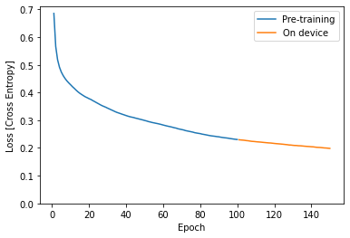
Run training for a few epochs to improve or personalize the model. In practice, you would run this additional training using data collected on the device. For simplicity, this example uses the same training data as the previous training step.

  train 
  
 = 
  
 interpreter 
 . 
 get_signature_runner 
 ( 
 "train" 
 ) 
 NUM_EPOCHS 
  
 = 
  
 50 
 BATCH_SIZE 
  
 = 
  
 100 
 more_epochs 
  
 = 
  
 np 
 . 
 arange 
 ( 
 epochs 
 [ 
 -1 
 ]+ 
 1 
 , 
  
 epochs 
 [ 
 -1 
 ] 
  
 + 
  
 NUM_EPOCHS 
  
 + 
  
 1 
 , 
  
 1 
 ) 
 more_losses 
  
 = 
  
 np 
 . 
 zeros 
 ( 
 [ 
 NUM_EPOCHS 
 ] 
 ) 
 for 
  
 i 
  
 in 
  
 range 
 ( 
 NUM_EPOCHS 
 ) 
 : 
  
 for 
  
 x 
 , 
 y 
  
 in 
  
 train_ds 
 : 
  
 result 
  
 = 
  
 train 
 ( 
 x 
 = 
 x 
 , 
  
 y 
 = 
 y 
 ) 
  
 more_losses 
 [ 
 i 
 ] 
  
 = 
  
 result 
 [ 
 'loss' 
 ] 
  
 if 
  
 ( 
 i 
  
 + 
  
 1 
 ) 
  
 % 
  
 10 
  
 == 
  
 0 
 : 
  
 print 
 ( 
 f 
 "Finished {i+1} epochs" 
 ) 
  
 print 
 ( 
 f 
 "  loss: {more_losses[i]:.3f}" 
 ) 
 
Finished 10 epochs
  loss&colon; 0.223
Finished 20 epochs
  loss&colon; 0.216
Finished 30 epochs
  loss&colon; 0.210
Finished 40 epochs
  loss&colon; 0.204
Finished 50 epochs
  loss&colon; 0.198
  plt 
 . 
 plot 
 ( 
 epochs 
 , 
  
 losses 
 , 
  
 label 
 = 
 ' 
 Pre 
 - 
 training 
 ' 
 ) 
 plt 
 . 
 plot 
 ( 
 more_epochs 
 , 
  
 more_losses 
 , 
  
 label 
 = 
 ' 
 On 
  
 device 
 ' 
 ) 
 plt 
 . 
 ylim 
 ([ 
 0 
 , 
  
 max 
 ( 
 plt 
 . 
 ylim 
 ())]) 
 plt 
 . 
 xlabel 
 ( 
 ' 
 Epoch 
 ' 
 ) 
 plt 
 . 
 ylabel 
 ( 
 ' 
 Loss 
  
 [ 
 Cross 
  
 Entropy 
 ] 
 ' 
 ) 
 plt 
 . 
 legend 
 (); 
 

png

Above you can see that the on-device training picks up exactly where the pretraining stopped.

Save the trained weights

When you complete a training run on a device, the model updates the set of weights it is using in memory. Using the save signature method you created in your LiteRT model, you can save these weights to a checkpoint file for later reuse and improve your model.

  save 
  
 = 
  
 interpreter 
 . 
 get_signature_runner 
 ( 
 "save" 
 ) 
 save 
 ( 
 checkpoint_path 
 = 
 np 
 . 
 array 
 ( 
 "/tmp/model.ckpt" 
 , 
  
 dtype 
 = 
 np 
 . 
 string_ 
 )) 
 
{'checkpoint_path'&colon; array(b'/tmp/model.ckpt', dtype=object)}

In your Android application, you can store the generated weights as a checkpoint file in the internal storage space allocated for your app.

  try 
  
 ( 
 Interpreter 
  
 interpreter 
  
 = 
  
 new 
  
 Interpreter 
 ( 
 modelBuffer 
 )) 
  
 { 
  
 // Conduct the training jobs. 
  
 // Export the trained weights as a checkpoint file. 
  
 File 
  
 outputFile 
  
 = 
  
 new 
  
 File 
 ( 
 getFilesDir 
 (), 
  
 "checkpoint.ckpt" 
 ); 
  
 Map<String 
 , 
  
 Object 
>  
 inputs 
  
 = 
  
 new 
  
 HashMap 
<> (); 
  
 inputs 
 . 
 put 
 ( 
 "checkpoint_path" 
 , 
  
 outputFile 
 . 
 getAbsolutePath 
 ()); 
  
 Map<String 
 , 
  
 Object 
>  
 outputs 
  
 = 
  
 new 
  
 HashMap 
<> (); 
  
 interpreter 
 . 
 runSignature 
 ( 
 inputs 
 , 
  
 outputs 
 , 
  
 "save" 
 ); 
 } 
 

Restore the trained weights

Any time you create an interpreter from a TFLite model, the interpreter will initially load the original model weights.

So after you've done some training and saved a checkpoint file, you'll need to run the restore signature method to load the checkpoint.

A good rule is "Anytime you create an Interpreter for a model, if the checkpoint exists, load it". If you need to reset the model to the baseline behavior, just delete the checkpoint and create a fresh interpreter.

 another_interpreter = tf.lite.Interpreter(model_content=tflite_model)
another_interpreter.allocate_tensors()

infer = another_interpreter.get_signature_runner("infer")
restore = another_interpreter.get_signature_runner("restore") 
  logits_before 
  
 = 
  
 infer 
 ( 
 x 
 = 
 train_images 
 [: 
 1 
 ])[ 
 ' 
 logits 
 ' 
 ][ 
 0 
 ] 
 # 
  
 Restore 
  
 the 
  
 trained 
  
 weights 
  
 from 
  
 / 
 tmp 
 / 
 model 
 . 
 ckpt 
 restore 
 ( 
 checkpoint_path 
 = 
 np 
 . 
 array 
 ( 
 "/tmp/model.ckpt" 
 , 
  
 dtype 
 = 
 np 
 . 
 string_ 
 )) 
 logits_after 
  
 = 
  
 infer 
 ( 
 x 
 = 
 train_images 
 [: 
 1 
 ])[ 
 ' 
 logits 
 ' 
 ][ 
 0 
 ] 
 compare_logits 
 ({ 
 ' 
 Before 
 ' 
 : 
  
 logits_before 
 , 
  
 ' 
 After 
 ' 
 : 
  
 logits_after 
 }) 
 

png

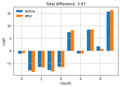
The checkpoint was generated by training and saving with TFLite. Above you can see that applying the checkpoint updates the behavior of the model.

In your Android app, you can restore the serialized, trained weights from the checkpoint file you stored earlier.

  try 
  
 ( 
 Interpreter 
  
 anotherInterpreter 
  
 = 
  
 new 
  
 Interpreter 
 ( 
 modelBuffer 
 )) 
  
 { 
  
 // Load the trained weights from the checkpoint file. 
  
 File 
  
 outputFile 
  
 = 
  
 new 
  
 File 
 ( 
 getFilesDir 
 (), 
  
 "checkpoint.ckpt" 
 ); 
  
 Map<String 
 , 
  
 Object 
>  
 inputs 
  
 = 
  
 new 
  
 HashMap 
<> (); 
  
 inputs 
 . 
 put 
 ( 
 "checkpoint_path" 
 , 
  
 outputFile 
 . 
 getAbsolutePath 
 ()); 
  
 Map<String 
 , 
  
 Object 
>  
 outputs 
  
 = 
  
 new 
  
 HashMap 
<> (); 
  
 anotherInterpreter 
 . 
 runSignature 
 ( 
 inputs 
 , 
  
 outputs 
 , 
  
 "restore" 
 ); 
 } 
 

Run Inference using trained weights

Once you have loaded previously saved weights from a checkpoint file, running the infer method uses those weights with your original model to improve predictions. After loading the saved weights, you can use the infer signature method as shown below.

 infer = another_interpreter.get_signature_runner("infer")
result = infer(x=test_images)
predictions = np.argmax(result["output"], axis=1)

true_labels = np.argmax(test_labels, axis=1) 
 result['output'].shape 
(10000, 10)

Plot the predicted labels.

  class_names 
  
 = 
  
 [ 
 'T-shirt/top', 'Trouser', 'Pullover', 'Dress', 'Coat', 
 'Sandal', 'Shirt', 'Sneaker', 'Bag', 'Ankle boot' 
 ] 
 def 
  
 plot 
 ( 
 images 
 , 
  
 predictions 
 , 
  
 true_labels 
 ) 
 : 
  
 plt 
 . 
 figure 
 ( 
 figsize 
 = 
 ( 
 10 
 , 
 10 
 )) 
  
 for 
  
 i 
  
 in 
  
 range 
 ( 
 25 
 ) 
 : 
  
 plt 
 . 
 subplot 
 ( 
 5 
 , 
 5 
 , 
 i 
 + 
 1 
 ) 
  
 plt 
 . 
 xticks 
 ( 
 [] 
 ) 
  
 plt 
 . 
 yticks 
 ( 
 [] 
 ) 
  
 plt 
 . 
 grid 
 ( 
 False 
 ) 
  
 plt 
 . 
 imshow 
 ( 
 images 
 [ 
 i 
 ] 
 , 
  
 cmap 
 = 
 plt 
 . 
 cm 
 . 
 binary 
 ) 
  
 color 
  
 = 
  
 'b' 
  
 if 
  
 predictions 
 [ 
 i 
 ] 
  
 == 
  
 true_labels 
 [ 
 i 
 ] 
  
 else 
  
 'r' 
  
 plt 
 . 
 xlabel 
 ( 
 class_names 
 [ 
 predictions[i 
 ] 
 ] 
 , 
  
 color 
 = 
 color 
 ) 
  
 plt 
 . 
 show 
 () 
 plot 
 ( 
 test_images 
 , 
  
 predictions 
 , 
  
 true_labels 
 ) 
 

png

 predictions.shape 
(10000,)

In your Android application, after restoring the trained weights, run the inferences based on the loaded data.

  try 
  
 ( 
 Interpreter 
  
 anotherInterpreter 
  
 = 
  
 new 
  
 Interpreter 
 ( 
 modelBuffer 
 )) 
  
 { 
  
 // Restore the weights from the checkpoint file. 
  
 int 
  
 NUM_TESTS 
  
 = 
  
 10 
 ; 
  
 FloatBuffer 
  
 testImages 
  
 = 
  
 FloatBuffer 
 . 
 allocateDirect 
 ( 
 NUM_TESTS 
  
 * 
  
 28 
  
 * 
  
 28 
 ). 
 order 
 ( 
 ByteOrder 
 . 
 nativeOrder 
 ()); 
  
 FloatBuffer 
  
 output 
  
 = 
  
 FloatBuffer 
 . 
 allocateDirect 
 ( 
 NUM_TESTS 
  
 * 
  
 10 
 ). 
 order 
 ( 
 ByteOrder 
 . 
 nativeOrder 
 ()); 
  
 // Fill the test data. 
  
 // Run the inference. 
  
 Map<String 
 , 
  
 Object 
>  
 inputs 
  
 = 
  
 new 
  
 HashMap 
<> (); 
  
 inputs 
 . 
 put 
 ( 
 "x" 
 , 
  
 testImages 
 . 
 rewind 
 ()); 
  
 Map<String 
 , 
  
 Object 
>  
 outputs 
  
 = 
  
 new 
  
 HashMap 
<> (); 
  
 outputs 
 . 
 put 
 ( 
 "output" 
 , 
  
 output 
 ); 
  
 anotherInterpreter 
 . 
 runSignature 
 ( 
 inputs 
 , 
  
 outputs 
 , 
  
 "infer" 
 ); 
  
 output 
 . 
 rewind 
 (); 
  
 // Process the result to get the final category values. 
  
 int 
 [] 
  
 testLabels 
  
 = 
  
 new 
  
 int 
 [ 
 NUM_TESTS 
 ] 
 ; 
  
 for 
  
 ( 
 int 
  
 i 
  
 = 
  
 0 
 ; 
  
 i 
 < 
 NUM_TESTS 
 ; 
  
 ++ 
 i 
 ) 
  
 { 
  
 int 
  
 index 
  
 = 
  
 0 
 ; 
  
 for 
  
 ( 
 int 
  
 j 
  
 = 
  
 1 
 ; 
  
 j 
 < 
 10 
 ; 
  
 ++ 
 j 
 ) 
  
 { 
  
 if 
  
 ( 
 output 
 . 
 get 
 ( 
 i 
  
 * 
  
 10 
  
 + 
  
 index 
 ) 
 < 
 output 
 . 
 get 
 ( 
 i 
  
 * 
  
 10 
  
 + 
  
 j 
 )) 
  
 index 
  
 = 
  
 testLabels 
 [ 
 j 
 ] 
 ; 
  
 } 
  
 testLabels 
 [ 
 i 
 ] 
  
 = 
  
 index 
 ; 
  
 } 
 } 
 

Congratulations! You now have built a LiteRT model that supports on-device training. For more coding details, check out the example implementation in the model personalization demo app .

If you are interested in learning more about image classification, check Keras classification tutorial in the TensorFlow official guide page. This tutorial is based on that exercise and provides more depth on the subject of classification.

Create a Mobile Website
View Site in Mobile | Classic
Share by: