
AI-generated Key Takeaways
-
GIS involves collecting, visualizing, and analyzing geographical or spatial data.
-
Geospatial data types commonly used in GIS are vector data (points, lines, polygons) and raster data (pixels representing values).
-
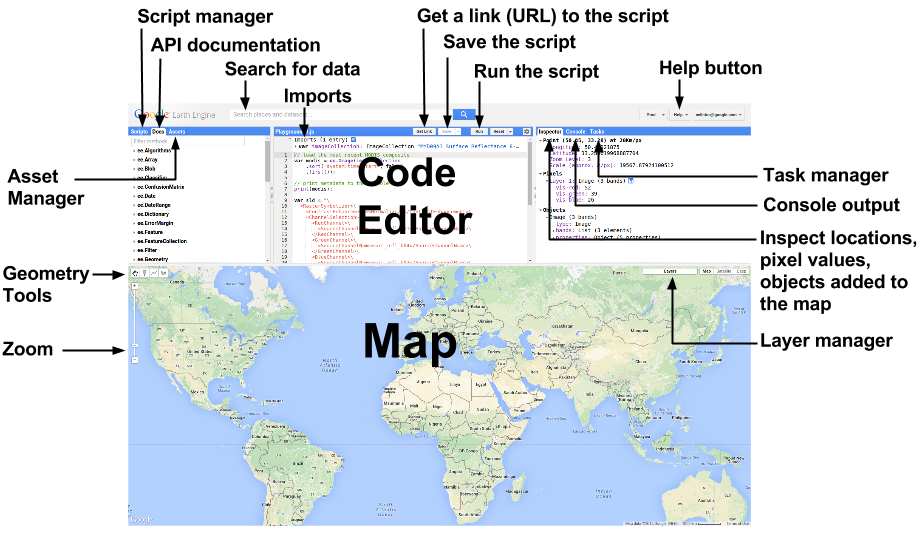
Google Earth Engine is a cloud-based platform for planetary scale geospatial analysis with a large archive of remote sensing data.
-
Basic Earth Engine functions include declaring variables, centering the map, displaying metadata, and adding layers.
-
Earth Engine supports various data types like strings, numbers, arrays, lists, dictionaries, geometries, features, images, and collections.
Introduction
GIS or Geographic Information System is the collection, visualization, and analysis of geographical or spatial data. In this section, we will cover the data types commonly used in GIS applications.
Vector data
Vector data represent objects on the Earth's surface using their longitude and latitude, as well as combinations of the pairs of coordinates (lines, polylines, polygons, etc.).
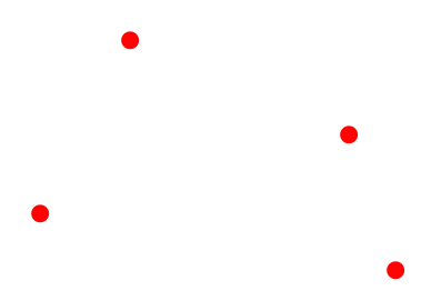
Point data
A pair of coordinates (longitude, latitude), that represents the location of points on the Earth's surface.
Example: Location of drop boxes, landmarks, etc.
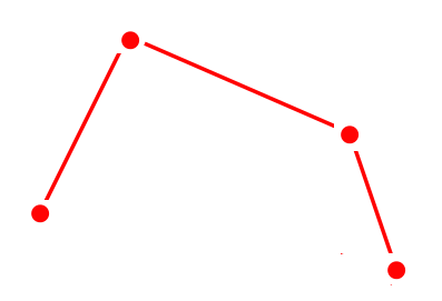
Lines
A series of points that represents a line (straight or otherwise) on the Earth's surface.
Example: Center of roads, rivers, etc.
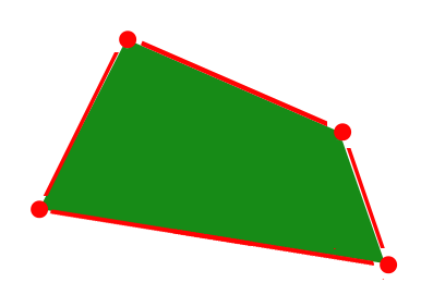
Polygons
A series of points (vertices) that define the outer edge of a region. Example: Outlines of cities, countries, continents, etc.
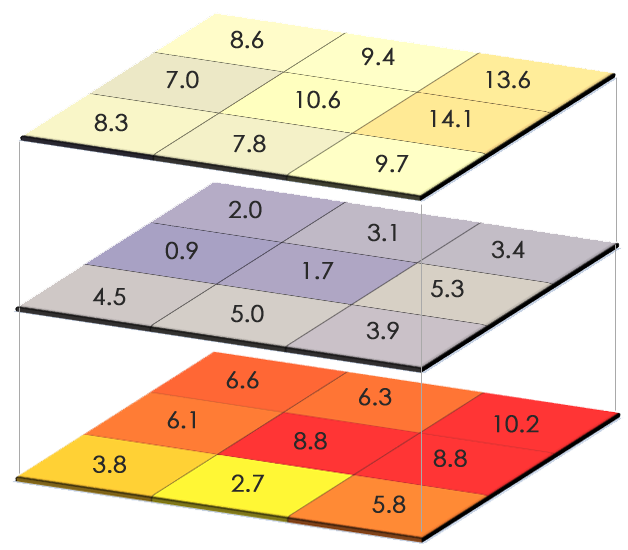
Raster data
Raster data represent objects/variables on the Earth's surface as a matrix of values, in the form of pixels, cells, or grids.
Layers and bands
A raster is an image with a matrix of values representing the values of some observed attribute. Bands of a raster correspond to different variables, usually using the same matrix structure.
Example: Spatial variability of temperature, elevation, rainfall, etc. over a region.
Conceptual figures sourced from GISGeography
The Google Earth Engine platform
What is Earth Engine?
- A cloud-based platform for planetary scale geospatial analysis
- Uses Google's computational resources to reduce processing time
- A massive archive of remote sensing data
Basic functions
Declaring variables
  var

 variableName

 =

 ee
 .
 ContainerType
 (
 value
 );
A container object (usually in the form ee.SomeVariableType
) is used to wrap a
native JavaScript object so that Google's servers can perform operations on it.
Centering the map
  Map
 .
 setCenter
 (
 long
 ,

 lat
 ,

 zoomLevel
 );
Zoom level varies from 0 (no zoom) to 20 (highest zoom level)
Displaying metadata
  print
 (
 variableName
 );
The print
operation is also useful for printing data and getting debugging
info. Note: You cannot print more than 5,000 elements at once.
Adding a layer to the map
  Map
 .
 addLayer
 (
 variableName
 );
Common Earth Engine data types
Strings
  var

 str

 =

 ee
 .
 String
 (
 'This is a string. Or is it? It is.'
 );
Numbers
  var

 num

 =

 ee
 .
 Number
 (
 5
 );
Arrays
  var

 arr

 =

 ee
 .
 Array
 ([[
 5
 ,

 2
 ,

 3
 ],

 [
 -
 2
 ,

 7
 ,

 10
 ],

 [
 6
 ,

 6
 ,

 9
 ]]);
Lists
  var

 lis

 =

 ee
 .
 List
 ([
 5
 ,

 'five'
 ,

 6
 ,

 'six'
 ]);
Dictionaries
  var

 dict

 =

 ee
 .
 Dictionary
 ({
 five
 :

 5
 ,

 six
 :

 6
 });
And the fun stuff...
-
ee.Geometry -
ee.Feature -
ee.FeatureCollection -
ee.Image -
ee.ImageCollection
Declaring geometries
Points
  var

 poi

 =

 ee
 .
 Geometry
 .
 Point
 (
 0
 ,

 45
 );
Multi points
  var

 multi

 =

 ee
 .
 Geometry
 .
 MultiPoint
 (
 0
 ,

 45
 ,

 5
 ,

 6
 ,

 70
 ,

 -
 56
 );
Line string
  var

 lineStr

 =

 ee
 .
 Geometry
 .
 LineString
 ([[
 0
 ,

 45
 ],

 [
 5
 ,

 6
 ],

 [
 70
 ,

 -
 56
 ]]);
Multi-line string
  var

 mLineStr

 =
 ee
 .
 Geometry
 .
 MultiLineString
 (

 [[[
 0
 ,

 45
 ],

 [
 5
 ,

 6
 ],

 [
 70
 ,

 -
 56
 ]],

 [[
 0
 ,

 -
 45
 ],

 [
 -
 5
 ,

 -
 6
 ],

 [
 -
 70
 ,

 56
 ]]]);
Linear ring
  var

 linRin

 =

 ee
 .
 Geometry
 .
 LinearRing
 (
 0
 ,

 45
 ,

 5
 ,

 6
 ,

 70
 ,

 -
 56
 ,

 0
 ,

 45
 );
Rectangle
  var

 rect

 =

 ee
 .
 Geometry
 .
 Rectangle
 (
 0
 ,

 0
 ,

 60
 ,

 30
 );
Polygon
  var

 poly

 =

 ee
 .
 Geometry
 .
 Polygon
 ([[[
 0
 ,

 0
 ],

 [
 6
 ,

 3
 ],

 [
 5
 ,

 5
 ],

 [
 -
 30
 ,

 2
 ],

 [
 0
 ,

 0
 ]]]);
Multi-polygon
  var

 multiPoly

 =
 ee
 .
 Geometry
 .
 MultiPolygon
 (

 [
 ee
 .
 Geometry
 .
 Polygon
 ([[
 0
 ,

 0
 ],

 [
 6
 ,

 3
 ],

 [
 5
 ,

 5
 ],

 [
 -
 30
 ,

 2
 ],

 [
 0
 ,

 0
 ]]),
 ee
 .
 Geometry
 .
 Polygon
 ([[
 0
 ,

 0
 ],

 [
 -
 6
 ,

 -
 3
 ],

 [
 -
 5
 ,

 -
 5
 ],

 [
 30
 ,

 -
 2
 ],

 [
 0
 ,

 0
 ]])]);
Features and FeatureCollections
- Features are geometries associated with specific properties.
- Feature collections are groups of features.
Functions and mapping
A function is a set of instructions to perform a specific task:
  function

 functionName
 (
 Arguments
 )

 {
 statements
 ;
 };
Calling a function
  var

 result

 =

 functionName
 (
 input
 );
Mapping a function over a collection
  var

 result

 =

 input
 .
 map
 (
 functionName
 );
Mapping a function over a collection applies the function to every element in the collection.
Common operations on geometries
Finding the area of a geometry
  var

 geoArea

 =

 geometry
 .
 area
 (
 maxError
 );
By default, all units in Earth Engine are in meters.
Finding the length of a line
  var

 linLen

 =

 lineString
 .
 length
 (
 maxError
 );
Finding the perimeter of a geometry
  var

 geoPeri

 =

 geometry
 .
 perimeter
 (
 maxError
 );
Reducing number of vertices in geometry
  var

 simpGeo

 =

 geometry
 .
 simplify
 (
 maxError
 );
Finding the centroid of a geometry
  var

 centrGeo

 =

 geometry
 .
 centroid
 (
 maxError
 );
Creating buffer around a geometry
  var

 buffGeo

 =

 geometry
 .
 buffer
 (
 radius
 ,

 maxError
 );
Finding the bounding rectangle of a geometry
  var

 bounGeo

 =

 geometry
 .
 bounds
 (
 maxError
 );
Finding the smallest polygon that can envelope a geometry
  var

 convexGeo

 =

 geometry
 .
 convexHull
 (
 maxError
 );
Finding common areas between two or more geometries
  var

 interGeo

 =

 geometry1
 .
 intersection
 (
 geometry2
 ,

 maxError
 );
Finding the area that includes two or more geometries
  var

 unGeo

 =

 geometry1
 .
 union
 (
 geometry2
 ,

 maxError
 );
Example: Geometry operations
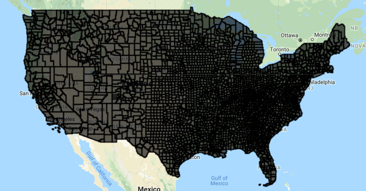
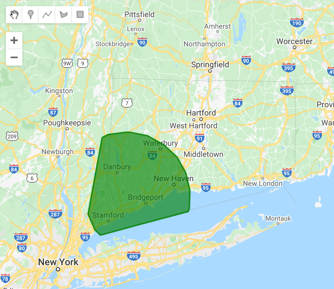
Let's run some these operations over the state of Connecticut, US using geometries of the public US counties feature collection available on Earth Engine:
1.We begin by zooming to the region of interest and loading/creating the geometries of interest by extracting them from the corresponding features.
  // Set map center over the state of CT.
 Map
 .
 setCenter
 (
 -
 72.6978
 ,

 41.6798
 ,

 8
 );
 // Load US county dataset.
 var

 countyData

 =

 ee
 .
 FeatureCollection
 (
 'TIGER/2018/Counties'
 );
 // Filter the counties that are in Connecticut (more on filters later).
 var

 countyConnect

 =

 countyData
 .
 filter
 (
 ee
 .
 Filter
 .
 eq
 (
 'STATEFP'
 ,

 '09'
 ));
 // Get the union of all the county geometries in Connecticut.
 var

 countyConnectDiss

 =

 countyConnect
 .
 union
 (
 100
 );
 // Create a circular area using the first county in the Connecticut
 // FeatureCollection.
 var

 circle

 =

 ee
 .
 Feature
 (
 countyConnect
 .
 first
 ())

 .
 geometry
 ().
 centroid
 (
 100
 ).
 buffer
 (
 50000
 ,

 100
 );
 // Add the layers to the map with a specified color and layer name.
 Map
 .
 addLayer
 (
 countyConnectDiss
 ,

 {
 color
 :

 'red'
 },

 'CT dissolved'
 );
 Map
 .
 addLayer
 (
 circle
 ,

 {
 color
 :

 'orange'
 },

 'Circle'
 );
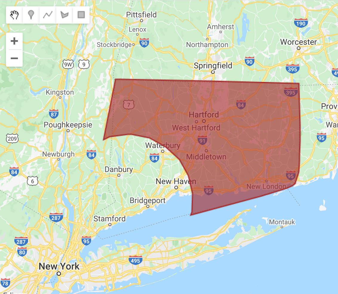
2.Using the bounds()
function, we can find the rectangle that emcompasses
the southernmost, westernmost, easternmost, and northernmost points of the
geometry.
  var

 bound

 =

 countyConnectDiss
 .
 geometry
 ().
 bounds
 (
 100
 );
 // Add the layer to the map with a specified color and layer name.
 Map
 .
 addLayer
 (
 bound
 ,

 {
 color
 :

 'yellow'
 },

 'Bounds'
 );
3.In the same vein, but not restricting ourselves to a rectangle, a convex
hull ( convexHull()
) is a polygon covering the extremities of the geometry.
  var

 convex

 =

 countyConnectDiss
 .
 geometry
 ().
 convexHull
 (
 100
 );
 // Add the layer to the map with a specified color and layer name.
 Map
 .
 addLayer
 (
 convex
 ,

 {
 color
 :

 'blue'
 },

 'Convex Hull'
 );
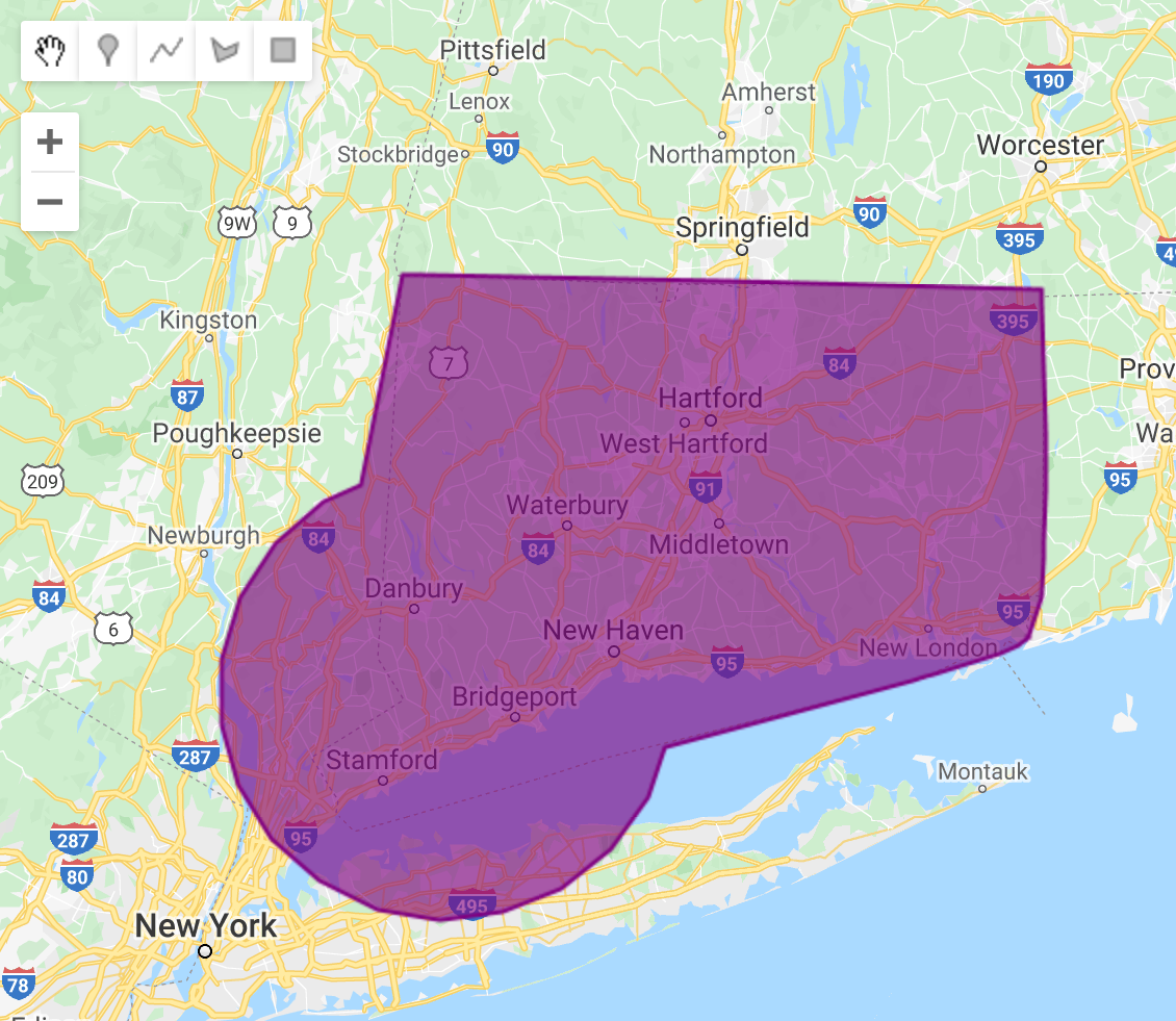
4.Moving on to some basic operations to combine multiple geometries, the
intersection ( intersection()
) is the area common to two or more geometries.
  var

 intersect

 =

 convex
 .
 intersection
 (
 circle
 ,

 100
 );
 // Add the layer to the map with a specified color and layer name.
 Map
 .
 addLayer
 (
 intersect
 ,

 {
 color
 :

 'green'
 },

 'Circle and convex intersection'
 );
5.The union ( union()
) is the area encompassing two or more features.
  // number is the maximum error in meters.
 var

 union

 =

 convex
 .
 union
 (
 circle
 ,

 100
 );
 // Add the layer to the map with a specified color and layer name.
 Map
 .
 addLayer
 (
 union
 ,

 {
 color
 :

 'purple'
 },

 'Circle and convex union'
 );
6.We can also find the spatial difference ( difference()
) between two
geometries.
  var

 diff

 =

 convex
 .
 difference
 (
 circle
 ,

 100
 );
 // Add the layer to the map with a specified color and layer name.
 Map
 .
 addLayer
 (
 diff
 ,

 {
 color
 :

 'brown'
 },

 'Circle and convex difference'
 );
| Difference | Union | Intersection |
|---|---|---|
 |
 |
 |
7.Finally, we can calculate and display the area, length, perimeter, etc. of our geometries.
  // Find area of feature.
 var

 ar

 =

 countyConnectDiss
 .
 geometry
 ().
 area
 (
 100
 );
 print
 (
 ar
 );
 // Find length of line geometry (You get zero since this is a polygon).
 var

 length

 =

 countyConnectDiss
 .
 geometry
 ().
 length
 (
 100
 );
 print
 (
 length
 );
 // Find perimeter of feature.
 var

 peri

 =

 countyConnectDiss
 .
 geometry
 ().
 perimeter
 (
 100
 );
 print
 (
 peri
 );
Example: Mapping over a feature collection
By mapping over a collection, one can apply the same operation on every element in a collection. For instance, let's run the same geometry operations on every county in Connecticut:
1.Similar to the previous example, we start by zooming into the map and loading the feature collection of CT counties.
  // Set map center over the state of CT.
 Map
 .
 setCenter
 (
 -
 72.6978
 ,

 41.6798
 ,

 8
 );
 // Load US county dataset.
 var

 countyData

 =

 ee
 .
 FeatureCollection
 (
 'TIGER/2018/Counties'
 );
 // Filter the counties that are in Connecticut.
 var

 countyConnect

 =

 countyData
 .
 filter
 (

 ee
 .
 Filter
 .
 eq
 (
 'STATEFP'
 ,

 '09'
 ));
 // Add the layer to the map with a specified color and layer name.
 Map
 .
 addLayer
 (
 countyConnect
 ,

 {
 color
 :

 'red'
 },

 'Original Collection'
 );
2.We define the function, which will perform the geometry operation on a feature. Try changing the operation being performed within the function to test what it does to the final output.
  function

 performMap
 (
 feature
 )

 {

 // Reduce number of vertices in geometry; the number is to specify maximum

 // error in meters. This is only for illustrative purposes, since Earth Engine

 // can handle up to 1 million vertices.

 var

 simple

 =

 feature
 .
 simplify
 (
 10000
 );

 // Find centroid of geometry.

 var

 center

 =

 simple
 .
 centroid
 (
 100
 );

 // Return buffer around geometry; the number represents the width of buffer,

 // in meters.

 return

 center
 .
 buffer
 (
 5000
 ,

 100
 );
 }
3.Finally, we map the defined function over all the features in the collection. This parallelization is generally much faster than performing operations sequentially over each element of the collection.
  var

 mappedCentroid

 =

 countyConnect
 .
 map
 (
 performMap
 );
 // Add the layer to the map with a specified color and layer name.
 Map
 .
 addLayer
 (
 mappedCentroid
 ,

 {
 color
 :

 'blue'
 },

 'Mapped buffed centroids'
 );
Operations on features
Creating a feature with a specific property value
  var

 feat

 =

 ee
 .
 Feature
 (
 geometry
 ,

 {
 Name
 :

 'featureName'
 ,

 Size
 :

 500
 });
Creating a feature from an existing feature, renaming a property
  var

 featNew

 =

 feature
 .
 select
 ([
 'name'
 ],

 [
 'descriptor'
 ]);
Extracting values of a property from a Feature
  var

 featVal

 =

 feature
 .
 get
 (
 'size'
 );
Example: Feature operations
Let's create a feature from scratch and play around with its properties:
  // Create geometry.
 var

 varGeometry

 =

 ee
 .
 Geometry
 .
 Polygon
 (
 0
 ,

 0
 ,

 40
 ,

 30
 ,

 20
 ,

 20
 ,

 0
 ,

 0
 );
 // Create feature from geometry.
 var

 varFeature

 =

 ee
 .
 Feature
 (
 varGeometry
 ,

 {

 name
 :

 [
 'Feature name'
 ,

 'Supreme'
 ],

 size
 :

 [
 500
 ,

 1000
 ]
 });
 // Get values of a property.
 var

 arr

 =

 varFeature
 .
 get
 (
 'size'
 );
 // Print variable.
 print
 (
 arr
 );
 // Select a subset of properties and rename them.
 var

 varFeaturenew

 =

 varFeature
 .
 select
 ([
 'name'
 ],

 [
 'descriptor'
 ]);
 // Print variable.
 print
 (
 varFeaturenew
 );
Filtering
Filtering by property values
  var

 bFilter

 =

 ee
 .
 Filter
 .
 eq
 (
 propertyName
 ,

 value
 );
or .neq , .gt , .gte , .lt , and .lte
Filtering based on maximum difference from a threshold
  var

 diffFilter

 =

 ee
 .
 Filter
 .
 maxDifference
 (
 threshold
 ,

 propertyName
 ,

 value
 );
Filtering by text property
  var

 txtFilter

 =

 ee
 .
 Filter
 .
 stringContains
 (
 propertyName
 ,

 stringValue
 );
or .stringStartsWith, and .stringEndsWith
Filtering by a value range
  var

 rangeFilter

 =

 ee
 .
 Filter
 .
 rangeContains
 (

 propertyName
 ,

 stringValue
 ,

 minValue
 ,

 maxValue
 );
Filtering by specific property values
  var

 listFilter

 =

 ee
 .
 Filter
 .
 listContains
 (

 propertyName
 ,

 value1
 ,

 propertyName2
 ,

 value2
 );
.inList to test against a list of values
Filtering by date range
  var

 dateFilter

 =

 ee
 .
 Filter
 .
 calendarRange
 (
 startDate
 ,

 stopDate
 );
Filtering by particular days of the year
  var

 dayFilter

 =

 ee
 .
 Filter
 .
 dayOfYear
 (
 startDay
 ,

 stopDay
 );
Filtering by a bounding area
  var

 boundsFilter

 =

 ee
 .
 Filter
 .
 bounds
 (
 geometryOrFeature
 );
Combining and inversing filters
  var

 newFilterAnd

 =

 ee
 .
 Filter
 .
 and
 (
 listOfFilters
 );
 var

 newFilterOr

 =

 ee
 .
 Filter
 .
 or
 (
 listOfFilters
 );
 var

 inverseFilter

 =

 ee
 .
 Filter
 .
 not
 (
 filter
 );
Operations on images
Selecting the bands of an image
  var

 band

 =

 image
 .
 select
 (
 bandName
 );
Creating masks
  var

 mask

 =

 image
 .
 eq
 (
 value
 );
or .neq or .gt or .gte or .lt or .lte
Applying image masks
  var

 masked

 =

 image
 .
 updateMask
 (
 mask
 );
Performing pixelwise calculations
  var

 results

 =

 image
 .
 add
 (
 value
 );
or .subtract , .multiply , .divide , .max , .min , .abs , .round , .floor , .ceil , .sqrt , .exp, .log, .log10, .sin , .cos , .tan , .sinh , .cosh , .tanh , .acos, .asin
Shift pixels of an image
  newImage

 =

 oldImage
 .
 leftShift
 (
 valueOfShift
 );
or .rightShift
Reducers
Reducers are objects in Earth Engine for data aggregation. They can be used for
aggregating across time, space, bands, properties, etc. Reducers range from
basic statistical indices (like ee.Reducer.mean()
, ee.Reducer.stdDev()
, ee.Reducer.max()
, etc.), to standard measures of covariance
(like ee.Reducer.linearFit()
, ee.Reducer.spearmansCorrelation()
, ee.Reducer.spearmansCorrelation()
, etc.), to descriptors of variable
distributions (like ee.Reducer.skew()
, ee.Reducer.frequencyHistogram()
, ee.Reducer.kurtosis()
, etc.). To get the first (or only) value for a property,
use ee.Reducer.first()
.
Reducing an image collection to an image
  var

 outputImage

 =

 imCollection
 .
 reduce
 (
 reducer
 );
Reducing an image to a statistic for an area of interest
  var

 outputDictionary

 =

 varImage
 .
 reduceRegion
 (
 reducer
 ,

 geometry
 ,

 scale
 );
Alternatively, reduceRegions
can be used to compute image statistics for all
elements of a collection at once:
  var

 outputCollection

 =

 varImage
 .
 reduceRegions
 (
 reducer
 ,

 collection
 ,

 scale
 );
Note that for large collections, this may be less efficient than mapping over
the collection and using reduceRegion
.
Applying a reducer to each element of a collection
  var

 outputDictionary

 =

 reduceColumns
 (
 reducer
 ,

 selectors
 );
Applying a reducer to the neighborhoods of each pixel
  var

 outputImage

 =

 reduceNeighborhood
 (
 reducer
 ,

 kernel
 );
Applying a reducer to each element of an array pixel
  var

 outputImage

 =

 arrayAccum
 (
 axis
 ,

 reducer
 );
Convert the properties of a vector into a raster
  var

 outputImage

 =

 reduceToImage
 (
 properties
 ,

 reducer
 );
Convert a raster into a vector
  var

 outputCollection

 =

 reduceToVectors
 (
 reducer
 );
Operations on image collections
Selecting the first n images in a collection (based on property)
  var

 selectedImages

 =

 imCollection
 .
 limit
 (
 n
 ,

 propertyName
 ,

 order
 );
Selecting images based on particular properties
  var

 selectedIm

 =

 imCollection
 .
 filterMetadata
 (
 propertyName
 ,

 operator
 ,

 value
 );
Operators include: "equals", "less_than", "greater_than", "not_equals", "not_less_than", "not_greater_than", "starts_with", "ends_with", "not_starts_with", "not_ends_with", "contains", "not_contains".
Selecting images within a date range
  var

 selectedIm

 =

 imCollection
 .
 filterDate
 (
 startDate
 ,

 stopDate
 );
Selecting images within a bounding geometry
  var

 selectedIm

 =

 imCollection
 .
 filterBounds
 (
 geometry
 );
Performing pixelwise calculations for all images in a collection
  var

 sumOfImages

 =

 imCollection
 .
 sum
 ();
or
product(),max(),min(),mean(),mode(),median(),count().
Alternatively, using reducers:
  var

 sumOfImages

 =

 imCollection
 .
 reduce
 (
 ee
 .
 Reducer
 .
 sum
 ());
Compositing images in collection with the last image on top
  var

 mosaicOfImages

 =

 imCollection
 .
 mosaic
 ();
Alternatively, using reducers:
  var

 sumOfImages

 =

 imCollection
 .
 reduce
 (
 ee
 .
 Reducer
 .
 first
 ());
Example: Image and image collection operations
Let's analyze images over a region of interest (the counties of Connecticut):
1.As before, we start by loading in the feature and image collections of interest.
  // Set map center over the state of CT.
 Map
 .
 setCenter
 (
 -
 72.6978
 ,

 41.6798
 ,

 8
 );
 // Load the MODIS MYD11A2 (8-day LST) image collection.
 var

 raw

 =

 ee
 .
 ImageCollection
 (
 'MODIS/006/MYD11A2'
 );
 // Load US county dataset.
 var

 countyData

 =

 ee
 .
 FeatureCollection
 (
 'TIGER/2018/Counties'
 );
 // Filter the counties that are in Connecticut.
 // This will be the region of interest for the image operations.
 var

 roi

 =

 countyData
 .
 filter
 (
 ee
 .
 Filter
 .
 eq
 (
 'STATEFP'
 ,

 '09'
 ));
 // Examine image collection.
 print
 (
 raw
 );
2.We select the bands and images in the collection we are interested in.
  // Select a band of the image collection using either indexing or band name.
 var

 bandSel1

 =

 raw
 .
 select
 (
 0
 );
 var

 bandSel2

 =

 raw
 .
 select
 (
 'LST_Day_1km'
 );
 // Filter the image collection by a date range.
 var

 filtered

 =

 raw
 .
 filterDate
 (
 '2002-12-30'
 ,

 '2004-4-27'
 );
 // Print filtered collection.
 print
 (
 filtered
 );
 // Limit the image collection to the first 50 elements.
 var

 limited

 =

 raw
 .
 limit
 (
 50
 );
 // Print collections.
 print
 (
 limited
 );
 print
 (
 bandSel1
 );
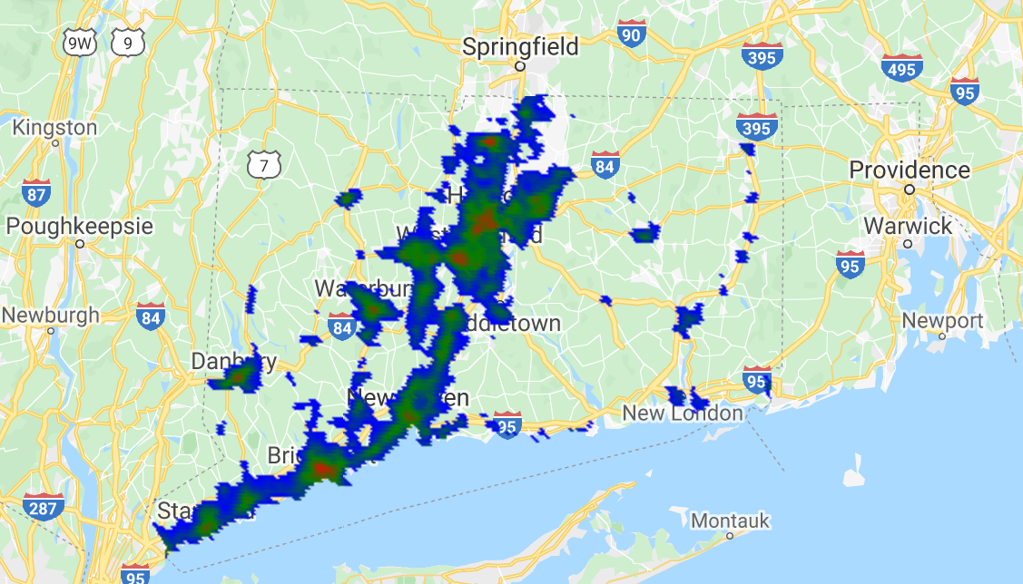
3.We calculate the mean of all the images in the collection, clip it to the geometry of interest and scale it to convert it from digital number to degree Celsius.
  // Calculate mean of all images (pixel-by-pixel) in the collection.
 var

 mean

 =

 bandSel1
 .
 mean
 ();
 // Isolate image to region of interest.
 var

 clipped

 =

 mean
 .
 clip
 (
 roi
 );
 // mathematical operation on image pixels to convert from digital number
 // of satellite observations to degree Celsius.
 var

 calculate

 =

 clipped
 .
 multiply
 (
 0.02
 ).
 subtract
 (
 273.15
 );
 // Add the layer to the map with a specified color palette and layer name.
 Map
 .
 addLayer
 (

 calculate
 ,

 {
 min
 :

 15
 ,

 max
 :

 20
 ,

 palette
 :

 [
 'blue'
 ,

 'green'
 ,

 'red'
 ]},

 'LST'
 );
4.We mask out parts of the image to display regions above and below certain temperature thresholds.
  // Select pixels in the image that are greater than 30.8.
 var

 mask

 =

 calculate
 .
 gt
 (
 18
 );
 // Add the mask to the map with a layer name.
 Map
 .
 addLayer
 (
 mask
 ,

 {},

 'mask'
 );
 // Use selected pixels to update the mask of the whole image.
 var

 masked

 =

 calculate
 .
 updateMask
 (
 mask
 );
 // Add the final layer to the map with a specified color palette and layer name.
 Map
 .
 addLayer
 (
 masked
 ,

 {
 min
 :

 18
 ,

 max
 :

 25
 ,

 palette
 :

 [
 'blue'
 ,

 'green'
 ,

 'red'
 ]},

 'LST_masked'
 );
Exporting data
Exporting a collection to Google Drive, Earth Engine Asset, or Google Cloud
  Export
 .
 image
 .
 toDrive
 ({

 collection
 :

 varImage
 ,

 description
 :

 'fileName'
 ,

 region
 :

 geometry
 ,

 scale
 :

 1000
 });
or
Export.image.toCloudStorage(),Export.image.toAsset(),Export.table.toDrive(),Export.table.toCloudStorage(),Export.video.toCloudStorage(),Export.video.toDrive().
Example: Exporting data
1.Define a function to find the mean value of pixels in each feature of a collection.
  // Function to find mean of pixels in region of interest.
 var

 getRegions

 =

 function
 (
 image
 )

 {

 // Load US county dataset.

 var

 countyData

 =

 ee
 .
 FeatureCollection
 (
 'TIGER/2018/Counties'
 );

 // Filter the counties that are in Connecticut.

 // This will be the region of interest for the operations.

 var

 roi
 =
 countyData
 .
 filter
 (
 ee
 .
 Filter
 .
 eq
 (
 'STATEFP'
 ,

 '09'
 ));

 return

 image
 .
 reduceRegions
 ({

 // Collection to run operation over.

 collection
 :

 roi
 ,

 // Calculate mean of all pixels in region.

 reducer
 :

 ee
 .
 Reducer
 .
 mean
 (),

 // Pixel resolution used for the calculations.

 scale
 :

 1000

 });
 };
2.Load image collection, filter collection to date range, select band of interest, calculate mean of all images in collection, and multiply by scaling factor.
  var

 image

 =

 ee
 .
 ImageCollection
 (
 'MODIS/MYD13A1'
 )

 .
 filterDate
 (
 '2002-07-08'
 ,

 '2017-07-08'
 )

 .
 select
 (
 'NDVI'
 )

 .
 mean
 ()

 .
 multiply
 (
 .0001
 );
 // Print final image.
 print
 (
 image
 );
 // Call function.
 var

 coll

 =

 getRegions
 (
 image
 );
3.Export the table created to your Google Drive.
  Export
 .
 table
 .
 toDrive
 ({

 collection
 :

 coll
 ,

 description
 :

 'NDVI_all'
 ,

 fileFormat
 :

 'CSV'
 });
 // Print final collection.
 print
 (
 coll
 );
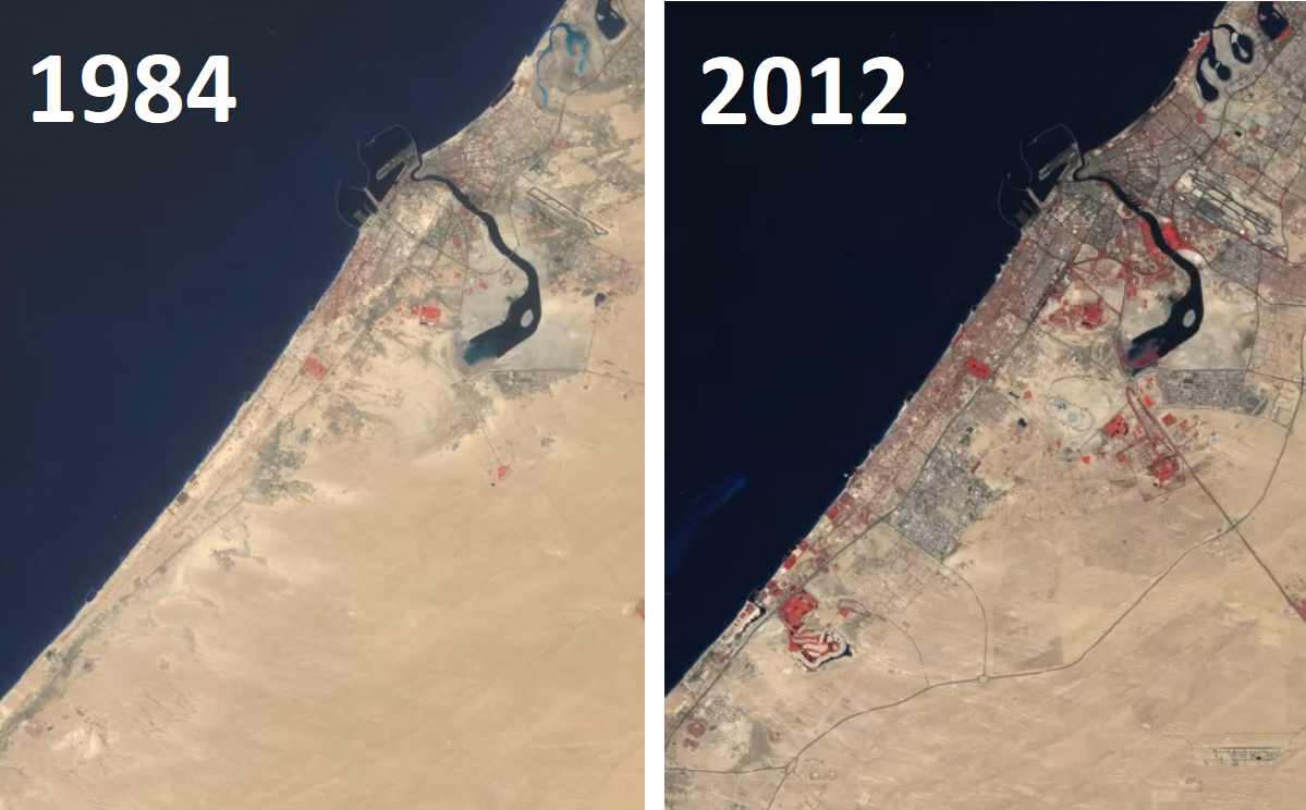
Bonus: Timelapse example
  // Timelapse example (based on google API example);
 // Create rectangle over Dubai.
 var

 geometry

 =

 ee
 .
 Geometry
 .
 Rectangle
 ([
 55.1
 ,

 25
 ,

 55.4
 ,

 25.4
 ]);
 // Add layer to map.
 Map
 .
 addLayer
 (
 geometry
 );
 // Load Landsat image collection.
 var

 allImages

 =

 ee
 .
 ImageCollection
 (
 'LANDSAT/LT05/C02/T1_TOA'
 )

 // Filter row and path such that they cover Dubai.

 .
 filter
 (
 ee
 .
 Filter
 .
 eq
 (
 'WRS_PATH'
 ,

 160
 ))

 .
 filter
 (
 ee
 .
 Filter
 .
 eq
 (
 'WRS_ROW'
 ,

 43
 ))

 // Filter cloudy scenes.

 .
 filter
 (
 ee
 .
 Filter
 .
 lt
 (
 'CLOUD_COVER'
 ,

 30
 ))

 // Get required years of imagery.

 .
 filterDate
 (
 '1984-01-01'
 ,

 '2012-12-30'
 )

 // Select 3-band imagery for the video.

 .
 select
 ([
 'B4'
 ,

 'B3'
 ,

 'B2'
 ])

 // Make the data 8-bit.

 .
 map
 (
 function
 (
 image
 )

 {

 return

 image
 .
 multiply
 (
 512
 ).
 uint8
 ();

 });
 Export
 .
 video
 .
 toDrive
 ({

 collection
 :

 allImages
 ,

 // Name of file.

 description
 :

 'dubaiTimelapse'
 ,

 // Quality of video.

 dimensions
 :

 720
 ,

 // FPS of video.

 framesPerSecond
 :

 8
 ,

 // Region of export.

 region
 :

 geometry
 });
Example applications
What can you do with Google Earth Engine?
- EE Population Explorer
- EE Ocean Time Series Investigator
- Global Surface UHI Explorer
- Stratifi - cloud-based stratification
- And hundreds more...