
AI-generated Key Takeaways
-
Learn how to calculate the fraction of a single land cover class within a specific region using Dynamic World data.
-
Discover how to summarize pixel counts for all land cover classes in a region using the
ee.Reducer.frequencyHistogram().unweighted()reducer. -
Understand how to export pixel count statistics as a CSV file to Google Drive.
A high resolution Land Use Land Cover (LULC) dataset like Dynamic World allows us to estimate the footprint of human activity on carbon cycles, biodiversity and other anthropogenic natural processes. Using the Dynamic World taxonomy, we can calculate and summarize statistics over any region. In this section, we will learn how to calculate the number of pixels for a single land cover class in a region as well as the distribution of pixel counts for all classes.
Note that summary statistics could be used to get class proportions for a stratified sample, but reference data would need to be collected in order to correct for biases and perform area estimation.
We continue from Part 1 of the Tutorial with the selected region of Dane County, Wisconsin. In this section, you will learn how to calculate the fraction of a single land cover class in this county as well as the pixel counts for all the classes.
Calculate the Fraction of a Single Class
Let's say we want to estimate what percentage of a region is built-up area. We start by creating a mode composite for the given time period.
  var

 counties

 =

 ee
 .
 FeatureCollection
 (
 'TIGER/2016/Counties'
 );
 var

 filtered

 =

 counties
 .
 filter
 (
 ee
 .
 Filter
 .
 eq
 (
 'NAMELSAD'
 ,

 'Dane County'
 ));
 var

 geometry

 =

 filtered
 .
 geometry
 ();
 Map
 .
 centerObject
 (
 geometry
 ,

 10
 );
 var

 startDate

 =

 '2020-01-01'
 ;
 var

 endDate

 =

 '2021-01-01'
 ;
 var

 dw

 =

 ee
 .
 ImageCollection
 (
 'GOOGLE/DYNAMICWORLD/V1'
 )

 .
 filterDate
 (
 startDate
 ,

 endDate
 )

 .
 filterBounds
 (
 geometry
 );
 // Create a mode composite.
 var

 classification

 =

 dw
 .
 select
 (
 'label'
 );
 var

 dwComposite

 =

 classification
 .
 reduce
 (
 ee
 .
 Reducer
 .
 mode
 ());
According to the Dynamic World taxonomy, the Built Area
class is
represented with the pixel value 6. We can use the boolean operator .eq()
to extract all pixels with that value.
  // Extract the Built Area class.
 var

 builtArea

 =

 dwComposite
 .
 eq
 (
 6
 );
The resulting builtArea
image is a binary image—with pixel value 1 where
the condition matched and 0 where it didn't. We can add both the composite
and the built area images to the Map to verify it.
  var

 dwVisParams

 =

 {

 min
 :

 0
 ,

 max
 :

 8
 ,

 palette
 :

 [

 '#419BDF'
 ,

 '#397D49'
 ,

 '#88B053'
 ,

 '#7A87C6'
 ,

 '#E49635'
 ,

 '#DFC35A'
 ,

 '#C4281B'
 ,

 '#A59B8F'
 ,

 '#B39FE1'

 ]
 };
 // Clip the composite and add it to the Map.
 Map
 .
 addLayer
 (
 dwComposite
 .
 clip
 (
 geometry
 ),

 dwVisParams
 ,

 'Classified Composite'
 );
 Map
 .
 addLayer
 (
 builtArea
 .
 clip
 (
 geometry
 ),

 {},

 'Built Areas'
 );
| Composite | Built Area Composite |
|---|---|
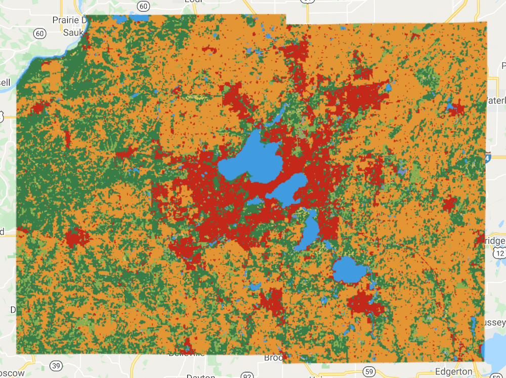 |
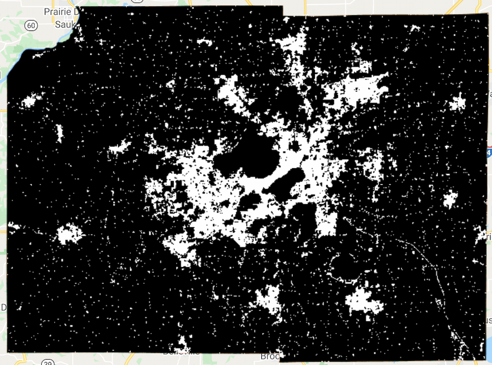 |
Dynamic World Composite and Extracted Built Area Image
Before proceeding further, it is helpful to rename our image bands so it is easier to keep track of them.
  var

 dwComposite

 =

 dwComposite
 .
 rename
 ([
 'classification'
 ]);
 var

 builtArea

 =

 builtArea
 .
 rename
 ([
 'built_area'
 ]);
To count pixels within a region, we can use the reduceRegion()
function with
the ee.Reducer.count()
reducer. We first count total pixels in the image. Then
we use the selfMask()
function to mask all 0 values and count the remaining
pixels.
  // Count all pixels.
 var

 statsTotal

 =

 builtArea
 .
 reduceRegion
 ({

 reducer
 :

 ee
 .
 Reducer
 .
 count
 (),

 geometry
 :

 geometry
 ,

 scale
 :

 10
 ,

 maxPixels
 :

 1e10

 });
 var

 totalPixels

 =

 statsTotal
 .
 get
 (
 'built_area'
 );
 // Mask 0 pixel values and count remaining pixels.
 var

 builtAreaMasked

 =

 builtArea
 .
 selfMask
 ();
 var

 statsMasked

 =

 builtAreaMasked
 .
 reduceRegion
 ({

 reducer
 :

 ee
 .
 Reducer
 .
 count
 (),

 geometry
 :

 geometry
 ,

 scale
 :

 10
 ,

 maxPixels
 :

 1e10

 });
 var

 builtAreaPixels

 =

 statsMasked
 .
 get
 (
 'built_area'
 );
 print
 (
 builtAreaPixels
 );
The last step is to calculate the built area fraction by dividing the total
built area pixels by total image pixels. We round off the number to 2 decimal
places using the format()
function and print the result.
  var

 fraction

 =

 (
 ee
 .
 Number
 (
 builtAreaPixels
 ).
 divide
 (
 totalPixels
 ))

 .
 multiply
 (
 100
 );
 print
 (
 'Percentage Built Area'
 ,

 fraction
 .
 format
 (
 '%.2f'
 ));
Summarizing Pixel Counts for All Classes
The method described in the previous section is useful for many applications,
but it can be limiting if you want to summarize the pixel counts for all the
classes. Instead, we can take the dwComposite
image and use another reducer
called ee.Reducer.frequencyHistogram()
. This reducer computes the counts for
all unique pixel values in the image. Note that this is a weighted reducer, so
it will count the pixels based on their overlap with the geometry. To match the
results we get from ee.Reducer.count()
, we can create an unweighted reducer by
calling unweighted()
on it. Learn more about Weighted Reducers
.
  var

 pixelCountStats

 =

 dwComposite
 .
 reduceRegion
 ({

 reducer
 :

 ee
 .
 Reducer
 .
 frequencyHistogram
 ().
 unweighted
 (),

 geometry
 :

 geometry
 ,

 scale
 :

 10
 ,

 maxPixels
 :

 1e10

 });
 var

 pixelCounts

 =

 ee
 .
 Dictionary
 (
 pixelCountStats
 .
 get
 (
 'classification'
 ));
 print
 (
 pixelCounts
 );
The result is a dictionary with pixel values as keys and pixel counts as values. We can rename the keys in the dictionary with the class names to make the results more readable.
  // Format the results to make it more readable.
 var

 classLabels

 =

 ee
 .
 List
 ([

 'water'
 ,

 'trees'
 ,

 'grass'
 ,

 'flooded_vegetation'
 ,

 'crops'
 ,

 'shrub_and_scrub'
 ,

 'built'
 ,

 'bare'
 ,

 'snow_and_ice'

 ]);
 // Rename keys with class names.
 var

 pixelCountsFormatted

 =

 pixelCounts
 .
 rename
 (

 pixelCounts
 .
 keys
 (),

 classLabels
 );
 print
 (
 pixelCountsFormatted
 );
If you are summarizing pixel counts over a large region, you may get a Computation Timed Outerror when you print the results. In such cases, you must export the results instead of printing them in the Console.
The pixel counts are stored in a dictionary. To export it, we have to convert
the dictionary to a Feature Collection. A simple solution is to create a
Feature Collection having a single feature with null geometry and set the
dictionary as its properties. This resulting collection can then be exported
using the Export.table.toDrive()
function. Run the script and click Run
to
start the Export. Once the Export task finishes, you will have a file named pixel_counts.csv
in your Google Drive with the result of the computation.
  // Create a Feature Collection.
 var

 exportFc

 =

 ee
 .
 FeatureCollection
 (

 ee
 .
 Feature
 (
 null
 ,

 pixelCountsFormatted
 ));
 // Export the results as a CSV file.
 Export
 .
 table
 .
 toDrive
 ({

 collection
 :

 exportFc
 ,

 description
 :

 'pixel_counts_export'
 ,

 folder
 :

 'earthengine'
 ,

 fileNamePrefix
 :

 'pixel_counts'
 ,

 fileFormat
 :

 'CSV'
 ,
 });
Summary
You learned different techniques to calculate statistics on the LULC composite image. We covered the method to extract pixels for a single class and calculate its fraction. The tutorial also showed how to summarize pixel counts of all classes in a region and export the results as a CSV file.
The pixel counts obtained through the method described here should be used with care. For accurate area estimates, it should be further refined by comparing against reference datasets and applying bias corrections.
The full script for this section can be accessed from this Code Editor link: https://code.earthengine.google.com/020bc4a2311777545bcb1d44d6f524be
In Part 3 of this tutorial, we will explore the probability time-series and use it to detect changes.
The data described in this tutorial were produced by Google, in partnership with the World Resources Institute and National Geographic Society and are provided under a CC-BY-4.0 Attribution license.