Change Detection in Google Earth Engine - The MAD Transformation (Part 3)

Author(s): mortcanty

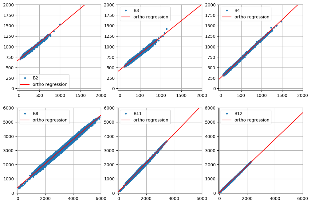
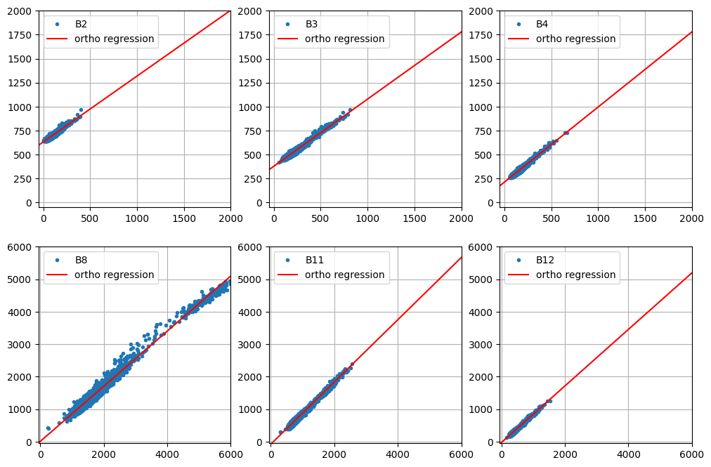
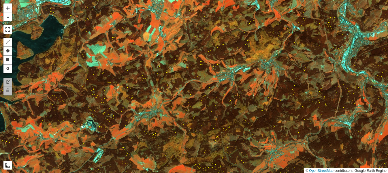
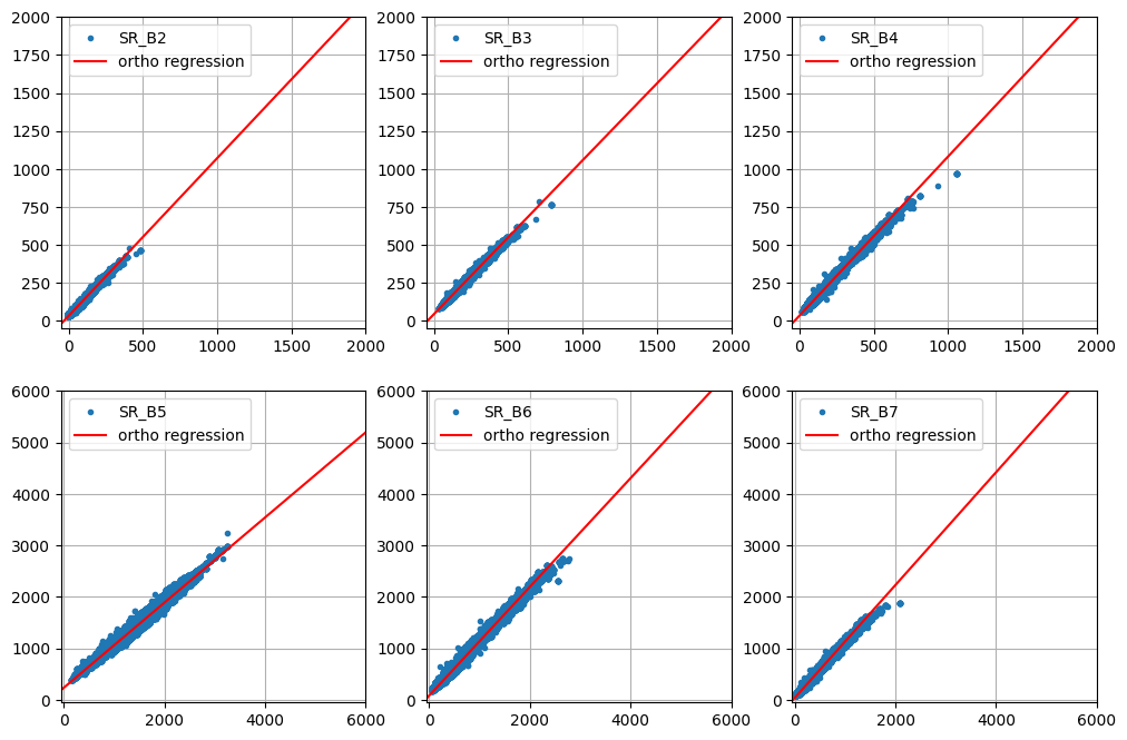
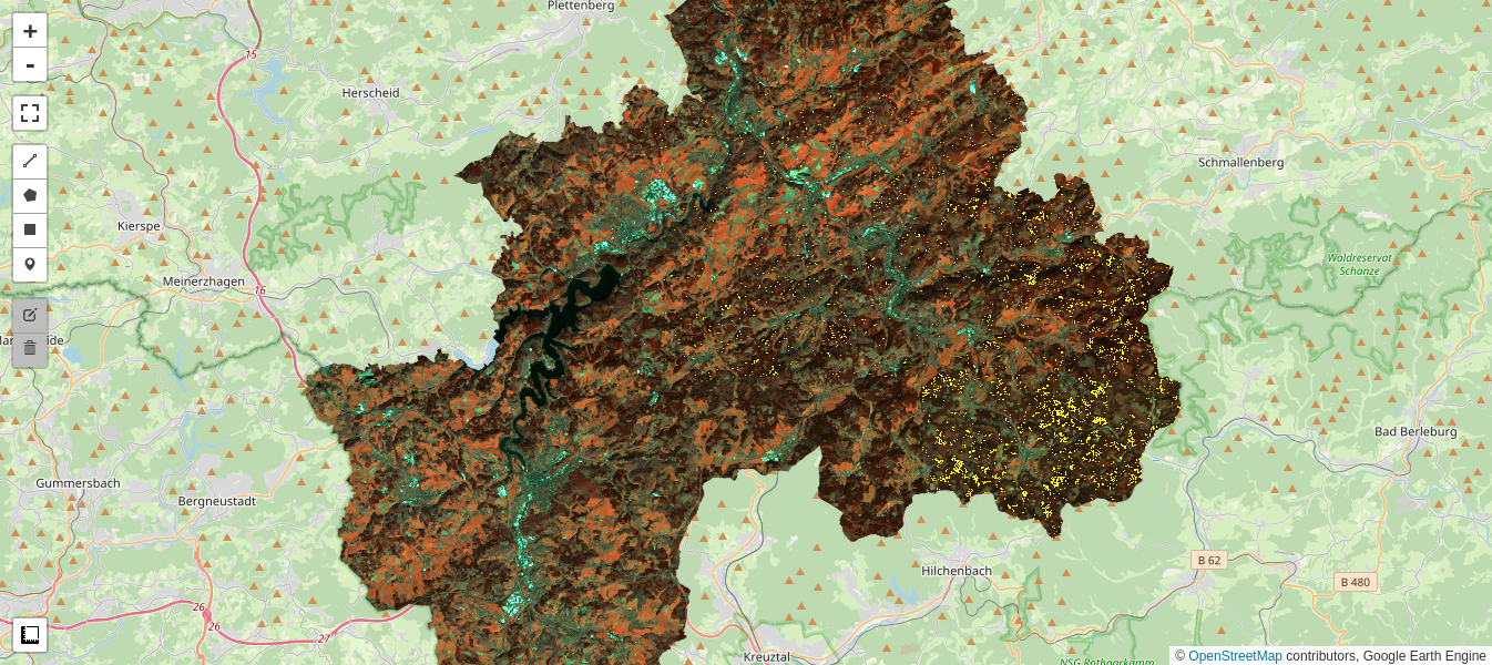
Test of pixel intensities across different image acquisitions requires that the received signals have similar radiometric scales. As we saw in Part 2 of the present tutorial, provided the iMAD algorithm converges satisfactorily, it will isolate the pixels which have not significantly changed in the two input images presented to it. A regression analysis on these no-change pixels can then determine how well the radiometric parameters of the two acquisitions compare. If, for instance, images that were corrected to absolute surface reflectance are examined in this way, we would expect a good match, i.e., a slope close to one and an intercept close to zero at all spectral wavelengths. In general, for uncalibrated or poorly corrected images, this will not be the case. Then, the regression coefficients can be applied to normalize one image (the target, say) to the other (the reference). This is a prerequisite, for example, for tracing features such as NDVI indices over a time series when the images have not been reduced to surface reflectances, see e.g., Gan et al. (2021) , or indeed for harmonizing the data from two different sensors of the same family, such as Landsat 8 with Landsat 9. In this final part of the GEE Change Detection Tutorial we'll have a closer look at this approach, which we'll refer to here as relative radiometric normalization . For more detailed treatment, see also Canty and Nielsen (2008) , Canty et al. (2004) , and Schroeder et al. (2006) . A different (but similar) method involving identification of so-called pseudoinvariant features is explained in another GEE community tutorial in this series.

Preliminaries

This tutorial will optionally export assets. Edit the following EXPORT_PATH variable to specify the location to store the assets. All assets that are needed to complete the tutorial are hosted by Earth Engine, but if you'd like to display assets that you export, replace paths as needed.

  # Enter your own export to assets path name here ----------- 
 EXPORT_PATH 
 = 
 'projects/YOUR_GEE_PROJECT_NAME/assets/imad/' 
 # ------------------------------------------------ 
 
  import 
  
 ee 
 ee 
 . 
 Authenticate 
 ( 
 auth_mode 
 = 
 'notebook' 
 ) 
 ee 
 . 
 Initialize 
 () 
 
  # Import other packages used in the tutorial 
 % 
 matplotlib 
 inline 
 import 
  
 geemap 
 import 
  
 numpy 
  
 as 
  
 np 
 import 
  
 random 
 , 
  
 time 
 import 
  
 matplotlib.pyplot 
  
 as 
  
 plt 
 from 
  
 scipy.stats 
  
 import 
 norm 
 , 
 chi2 
 from 
  
 pprint 
  
 import 
 pprint 
 # for pretty printing 
 

Routines from Parts 1 and 2

  def 
  
 trunc 
 ( 
 values 
 , 
 dec 
 = 
 3 
 ): 
  
 '''Truncate a 1-D array to dec decimal places.''' 
 return 
 np 
 . 
 trunc 
 ( 
 values 
 * 
 10 
 ** 
 dec 
 ) 
 / 
 ( 
 10 
 ** 
 dec 
 ) 
 # Display an image in a one percent linear stretch. 
 def 
  
 display_ls 
 ( 
 image 
 , 
 map 
 , 
 name 
 , 
 centered 
 = 
 False 
 ): 
 bns 
 = 
 image 
 . 
 bandNames 
 () 
 . 
 length 
 () 
 . 
 getInfo 
 () 
 if 
 bns 
 == 
 3 
 : 
 image 
 = 
 image 
 . 
 rename 
 ( 
 'B1' 
 , 
 'B2' 
 , 
 'B3' 
 ) 
 pb_99 
 = 
 [ 
 'B1_p99' 
 , 
 'B2_p99' 
 , 
 'B3_p99' 
 ] 
 pb_1 
 = 
 [ 
 'B1_p1' 
 , 
 'B2_p1' 
 , 
 'B3_p1' 
 ] 
 img 
 = 
 ee 
 . 
 Image 
 . 
 rgb 
 ( 
 image 
 . 
 select 
 ( 
 'B1' 
 ), 
 image 
 . 
 select 
 ( 
 'B2' 
 ), 
 image 
 . 
 select 
 ( 
 'B3' 
 )) 
 else 
 : 
 image 
 = 
 image 
 . 
 rename 
 ( 
 'B1' 
 ) 
 pb_99 
 = 
 [ 
 'B1_p99' 
 ] 
 pb_1 
 = 
 [ 
 'B1_p1' 
 ] 
 img 
 = 
 image 
 . 
 select 
 ( 
 'B1' 
 ) 
 percentiles 
 = 
 image 
 . 
 reduceRegion 
 ( 
 ee 
 . 
 Reducer 
 . 
 percentile 
 ([ 
 1 
 , 
 99 
 ]), 
 maxPixels 
 = 
 1e11 
 ) 
 mx 
 = 
 percentiles 
 . 
 values 
 ( 
 pb_99 
 ) 
 if 
 centered 
 : 
 mn 
 = 
 ee 
 . 
 Array 
 ( 
 mx 
 ) 
 . 
 multiply 
 ( 
 - 
 1 
 ) 
 . 
 toList 
 () 
 else 
 : 
 mn 
 = 
 percentiles 
 . 
 values 
 ( 
 pb_1 
 ) 
 map 
 . 
 addLayer 
 ( 
 img 
 , 
 { 
 'min' 
 : 
 mn 
 , 
 'max' 
 : 
 mx 
 }, 
 name 
 ) 
 def 
  
 covarw 
 ( 
 image 
 , 
 weights 
 = 
 None 
 , 
 scale 
 = 
 20 
 , 
 maxPixels 
 = 
 1e10 
 ): 
  
 '''Return the centered image and its weighted covariance matrix.''' 
 try 
 : 
 geometry 
 = 
 image 
 . 
 geometry 
 () 
 bandNames 
 = 
 image 
 . 
 bandNames 
 () 
 N 
 = 
 bandNames 
 . 
 length 
 () 
 if 
 weights 
 is 
 None 
 : 
 weights 
 = 
 image 
 . 
 constant 
 ( 
 1 
 ) 
 weightsImage 
 = 
 image 
 . 
 multiply 
 ( 
 ee 
 . 
 Image 
 . 
 constant 
 ( 
 0 
 )) 
 . 
 add 
 ( 
 weights 
 ) 
 means 
 = 
 image 
 . 
 addBands 
 ( 
 weightsImage 
 ) 
\ . 
 reduceRegion 
 ( 
 ee 
 . 
 Reducer 
 . 
 mean 
 () 
 . 
 repeat 
 ( 
 N 
 ) 
 . 
 splitWeights 
 (), 
 scale 
 = 
 scale 
 , 
 maxPixels 
 = 
 maxPixels 
 ) 
\ . 
 toArray 
 () 
\ . 
 project 
 ([ 
 1 
 ]) 
 centered 
 = 
 image 
 . 
 toArray 
 () 
 . 
 subtract 
 ( 
 means 
 ) 
 B1 
 = 
 centered 
 . 
 bandNames 
 () 
 . 
 get 
 ( 
 0 
 ) 
 b1 
 = 
 weights 
 . 
 bandNames 
 () 
 . 
 get 
 ( 
 0 
 ) 
 nPixels 
 = 
 ee 
 . 
 Number 
 ( 
 centered 
 . 
 reduceRegion 
 ( 
 ee 
 . 
 Reducer 
 . 
 count 
 (), 
 scale 
 = 
 scale 
 , 
 maxPixels 
 = 
 maxPixels 
 ) 
 . 
 get 
 ( 
 B1 
 )) 
 sumWeights 
 = 
 ee 
 . 
 Number 
 ( 
 weights 
 . 
 reduceRegion 
 ( 
 ee 
 . 
 Reducer 
 . 
 sum 
 (), 
 geometry 
 = 
 geometry 
 , 
 scale 
 = 
 scale 
 , 
 maxPixels 
 = 
 maxPixels 
 ) 
 . 
 get 
 ( 
 b1 
 )) 
 covw 
 = 
 centered 
 . 
 multiply 
 ( 
 weights 
 . 
 sqrt 
 ()) 
\ . 
 toArray 
 () 
\ . 
 reduceRegion 
 ( 
 ee 
 . 
 Reducer 
 . 
 centeredCovariance 
 (), 
 geometry 
 = 
 geometry 
 , 
 scale 
 = 
 scale 
 , 
 maxPixels 
 = 
 maxPixels 
 ) 
\ . 
 get 
 ( 
 'array' 
 ) 
 covw 
 = 
 ee 
 . 
 Array 
 ( 
 covw 
 ) 
 . 
 multiply 
 ( 
 nPixels 
 ) 
 . 
 divide 
 ( 
 sumWeights 
 ) 
 return 
 ( 
 centered 
 . 
 arrayFlatten 
 ([ 
 bandNames 
 ]), 
 covw 
 ) 
 except 
 Exception 
 as 
 e 
 : 
 print 
 ( 
 'Error: 
 %s 
 ' 
 % 
 e 
 ) 
 def 
  
 corr 
 ( 
 cov 
 ): 
  
 '''Transform covariance matrix to correlation matrix.''' 
 # Diagonal matrix of inverse sigmas. 
 sInv 
 = 
 cov 
 . 
 matrixDiagonal 
 () 
 . 
 sqrt 
 () 
 . 
 matrixToDiag 
 () 
 . 
 matrixInverse 
 () 
 # Transform. 
 corr 
 = 
 sInv 
 . 
 matrixMultiply 
 ( 
 cov 
 ) 
 . 
 matrixMultiply 
 ( 
 sInv 
 ) 
 . 
 getInfo 
 () 
 # Truncate. 
 return 
 [ 
 list 
 ( 
 map 
 ( 
 trunc 
 , 
 corr 
 [ 
 i 
 ])) 
 for 
 i 
 in 
 range 
 ( 
 len 
 ( 
 corr 
 ))] 
 def 
  
 geneiv 
 ( 
 C 
 , 
 B 
 ): 
  
 '''Return the eigenvalues and eigenvectors of the generalized eigenproblem 
 C*X = lambda*B*X''' 
 try 
 : 
 C 
 = 
 ee 
 . 
 Array 
 ( 
 C 
 ) 
 B 
 = 
 ee 
 . 
 Array 
 ( 
 B 
 ) 
 #  Li = choldc(B)^-1 
 Li 
 = 
 ee 
 . 
 Array 
 ( 
 B 
 . 
 matrixCholeskyDecomposition 
 () 
 . 
 get 
 ( 
 'L' 
 )) 
 . 
 matrixInverse 
 () 
 # Solve symmetric, ordinary eigenproblem Li*C*Li^T*x = lambda*x 
 Xa 
 = 
 Li 
 . 
 matrixMultiply 
 ( 
 C 
 ) 
\ . 
 matrixMultiply 
 ( 
 Li 
 . 
 matrixTranspose 
 ()) 
\ . 
 eigen 
 () 
 # Eigenvalues as a row vector. 
 lambdas 
 = 
 Xa 
 . 
 slice 
 ( 
 1 
 , 
 0 
 , 
 1 
 ) 
 . 
 matrixTranspose 
 () 
 # Eigenvectors as columns. 
 X 
 = 
 Xa 
 . 
 slice 
 ( 
 1 
 , 
 1 
 ) 
 . 
 matrixTranspose 
 () 
 # Generalized eigenvectors as columns, Li^T*X 
 eigenvecs 
 = 
 Li 
 . 
 matrixTranspose 
 () 
 . 
 matrixMultiply 
 ( 
 X 
 ) 
 return 
 ( 
 lambdas 
 , 
 eigenvecs 
 ) 
 except 
 Exception 
 as 
 e 
 : 
 print 
 ( 
 'Error: 
 %s 
 ' 
 % 
 e 
 ) 
 # Collect a Sentinel-2 image pair. 
 def 
  
 collect 
 ( 
 aoi 
 , 
 t1a 
 , 
 t1b 
 , 
 t2a 
 , 
 t2b 
 , 
 coll1 
 , 
 coll2 
 = 
 None 
 ): 
 try 
 : 
 if 
 coll2 
 == 
 None 
 : 
 coll2 
 = 
 coll1 
 im1 
 = 
 ee 
 . 
 Image 
 ( 
 ee 
 . 
 ImageCollection 
 ( 
 coll1 
 ) 
 . 
 filterBounds 
 ( 
 aoi 
 ) 
 . 
 filterDate 
 ( 
 ee 
 . 
 Date 
 ( 
 t1a 
 ), 
 ee 
 . 
 Date 
 ( 
 t1b 
 )) 
 . 
 filter 
 ( 
 ee 
 . 
 Filter 
 . 
 contains 
 ( 
 rightValue 
 = 
 aoi 
 , 
 leftField 
 = 
 '.geo' 
 )) 
 . 
 sort 
 ( 
 'CLOUDY_PIXEL_PERCENTAGE' 
 ) 
 . 
 sort 
 ( 
 'CLOUD_COVER_LAND' 
 ) 
 . 
 first 
 () 
 . 
 clip 
 ( 
 aoi 
 ) 
 ) 
 im2 
 = 
 ee 
 . 
 Image 
 ( 
 ee 
 . 
 ImageCollection 
 ( 
 coll2 
 ) 
 . 
 filterBounds 
 ( 
 aoi 
 ) 
 . 
 filterDate 
 ( 
 ee 
 . 
 Date 
 ( 
 t2a 
 ), 
 ee 
 . 
 Date 
 ( 
 t2b 
 )) 
 . 
 filter 
 ( 
 ee 
 . 
 Filter 
 . 
 contains 
 ( 
 rightValue 
 = 
 aoi 
 , 
 leftField 
 = 
 '.geo' 
 )) 
 . 
 sort 
 ( 
 'CLOUDY_PIXEL_PERCENTAGE' 
 ) 
 . 
 sort 
 ( 
 'CLOUD_COVER_LAND' 
 ) 
 . 
 first 
 () 
 . 
 clip 
 ( 
 aoi 
 ) 
 ) 
 timestamp 
 = 
 im1 
 . 
 date 
 () 
 . 
 format 
 ( 
 'E MMM dd HH:mm:ss YYYY' 
 ) 
 print 
 ( 
 timestamp 
 . 
 getInfo 
 ()) 
 timestamp 
 = 
 im2 
 . 
 date 
 () 
 . 
 format 
 ( 
 'E MMM dd HH:mm:ss YYYY' 
 ) 
 print 
 ( 
 timestamp 
 . 
 getInfo 
 ()) 
 return 
 ( 
 im1 
 , 
 im2 
 ) 
 except 
 Exception 
 as 
 e 
 : 
 print 
 ( 
 'Error: 
 %s 
 ' 
 % 
 e 
 ) 
 def 
  
 chi2cdf 
 ( 
 Z 
 , 
 df 
 ): 
  
 '''Chi-square cumulative distribution function with df degrees of freedom.''' 
 return 
 ee 
 . 
 Image 
 ( 
 Z 
 . 
 divide 
 ( 
 2 
 )) 
 . 
 gammainc 
 ( 
 ee 
 . 
 Number 
 ( 
 df 
 ) 
 . 
 divide 
 ( 
 2 
 )) 
 def 
  
 imad 
 ( 
 current 
 , 
 prev 
 ): 
  
 '''Iterator function for iMAD.''' 
 done 
 = 
 ee 
 . 
 Number 
 ( 
 ee 
 . 
 Dictionary 
 ( 
 prev 
 ) 
 . 
 get 
 ( 
 'done' 
 )) 
 return 
 ee 
 . 
 Algorithms 
 . 
 If 
 ( 
 done 
 , 
 prev 
 , 
 imad1 
 ( 
 current 
 , 
 prev 
 )) 
 def 
  
 imad1 
 ( 
 current 
 , 
 prev 
 ): 
  
 '''Iteratively re-weighted MAD.''' 
 image 
 = 
 ee 
 . 
 Image 
 ( 
 ee 
 . 
 Dictionary 
 ( 
 prev 
 ) 
 . 
 get 
 ( 
 'image' 
 )) 
 Z 
 = 
 ee 
 . 
 Image 
 ( 
 ee 
 . 
 Dictionary 
 ( 
 prev 
 ) 
 . 
 get 
 ( 
 'Z' 
 )) 
 allrhos 
 = 
 ee 
 . 
 List 
 ( 
 ee 
 . 
 Dictionary 
 ( 
 prev 
 ) 
 . 
 get 
 ( 
 'allrhos' 
 )) 
 nBands 
 = 
 image 
 . 
 bandNames 
 () 
 . 
 length 
 () 
 . 
 divide 
 ( 
 2 
 ) 
 weights 
 = 
 chi2cdf 
 ( 
 Z 
 , 
 nBands 
 ) 
 . 
 subtract 
 ( 
 1 
 ) 
 . 
 multiply 
 ( 
 - 
 1 
 ) 
 scale 
 = 
 ee 
 . 
 Dictionary 
 ( 
 prev 
 ) 
 . 
 getNumber 
 ( 
 'scale' 
 ) 
 niter 
 = 
 ee 
 . 
 Dictionary 
 ( 
 prev 
 ) 
 . 
 getNumber 
 ( 
 'niter' 
 ) 
 # Weighted stacked image and weighted covariance matrix. 
 centeredImage 
 , 
 covarArray 
 = 
 covarw 
 ( 
 image 
 , 
 weights 
 , 
 scale 
 ) 
 bNames 
 = 
 centeredImage 
 . 
 bandNames 
 () 
 bNames1 
 = 
 bNames 
 . 
 slice 
 ( 
 0 
 , 
 nBands 
 ) 
 bNames2 
 = 
 bNames 
 . 
 slice 
 ( 
 nBands 
 ) 
 centeredImage1 
 = 
 centeredImage 
 . 
 select 
 ( 
 bNames1 
 ) 
 centeredImage2 
 = 
 centeredImage 
 . 
 select 
 ( 
 bNames2 
 ) 
 s11 
 = 
 covarArray 
 . 
 slice 
 ( 
 0 
 , 
 0 
 , 
 nBands 
 ) 
 . 
 slice 
 ( 
 1 
 , 
 0 
 , 
 nBands 
 ) 
 s22 
 = 
 covarArray 
 . 
 slice 
 ( 
 0 
 , 
 nBands 
 ) 
 . 
 slice 
 ( 
 1 
 , 
 nBands 
 ) 
 s12 
 = 
 covarArray 
 . 
 slice 
 ( 
 0 
 , 
 0 
 , 
 nBands 
 ) 
 . 
 slice 
 ( 
 1 
 , 
 nBands 
 ) 
 s21 
 = 
 covarArray 
 . 
 slice 
 ( 
 0 
 , 
 nBands 
 ) 
 . 
 slice 
 ( 
 1 
 , 
 0 
 , 
 nBands 
 ) 
 c1 
 = 
 s12 
 . 
 matrixMultiply 
 ( 
 s22 
 . 
 matrixInverse 
 ()) 
 . 
 matrixMultiply 
 ( 
 s21 
 ) 
 b1 
 = 
 s11 
 c2 
 = 
 s21 
 . 
 matrixMultiply 
 ( 
 s11 
 . 
 matrixInverse 
 ()) 
 . 
 matrixMultiply 
 ( 
 s12 
 ) 
 b2 
 = 
 s22 
 # Solution of generalized eigenproblems. 
 lambdas 
 , 
 A 
 = 
 geneiv 
 ( 
 c1 
 , 
 b1 
 ) 
 _ 
 , 
 B 
 = 
 geneiv 
 ( 
 c2 
 , 
 b2 
 ) 
 rhos 
 = 
 lambdas 
 . 
 sqrt 
 () 
 . 
 project 
 ( 
 ee 
 . 
 List 
 ([ 
 1 
 ])) 
 # Test for convergence. 
 lastrhos 
 = 
 ee 
 . 
 Array 
 ( 
 allrhos 
 . 
 get 
 ( 
 - 
 1 
 )) 
 done 
 = 
 rhos 
 . 
 subtract 
 ( 
 lastrhos 
 ) 
\ . 
 abs 
 () 
\ . 
 reduce 
 ( 
 ee 
 . 
 Reducer 
 . 
 max 
 (), 
 ee 
 . 
 List 
 ([ 
 0 
 ])) 
\ . 
 lt 
 ( 
 ee 
 . 
 Number 
 ( 
 0.0001 
 )) 
\ . 
 toList 
 () 
\ . 
 get 
 ( 
 0 
 ) 
 allrhos 
 = 
 allrhos 
 . 
 cat 
 ([ 
 rhos 
 . 
 toList 
 ()]) 
 # MAD variances. 
 sigma2s 
 = 
 rhos 
 . 
 subtract 
 ( 
 1 
 ) 
 . 
 multiply 
 ( 
 - 
 2 
 ) 
 . 
 toList 
 () 
 sigma2s 
 = 
 ee 
 . 
 Image 
 . 
 constant 
 ( 
 sigma2s 
 ) 
 # Ensure sum of positive correlations between X and U is positive. 
 tmp 
 = 
 s11 
 . 
 matrixDiagonal 
 () 
 . 
 sqrt 
 () 
 ones 
 = 
 tmp 
 . 
 multiply 
 ( 
 0 
 ) 
 . 
 add 
 ( 
 1 
 ) 
 tmp 
 = 
 ones 
 . 
 divide 
 ( 
 tmp 
 ) 
 . 
 matrixToDiag 
 () 
 s 
 = 
 tmp 
 . 
 matrixMultiply 
 ( 
 s11 
 ) 
 . 
 matrixMultiply 
 ( 
 A 
 ) 
 . 
 reduce 
 ( 
 ee 
 . 
 Reducer 
 . 
 sum 
 (), 
 [ 
 0 
 ]) 
 . 
 transpose 
 () 
 A 
 = 
 A 
 . 
 matrixMultiply 
 ( 
 s 
 . 
 divide 
 ( 
 s 
 . 
 abs 
 ()) 
 . 
 matrixToDiag 
 ()) 
 # Ensure positive correlation. 
 tmp 
 = 
 A 
 . 
 transpose 
 () 
 . 
 matrixMultiply 
 ( 
 s12 
 ) 
 . 
 matrixMultiply 
 ( 
 B 
 ) 
 . 
 matrixDiagonal 
 () 
 tmp 
 = 
 tmp 
 . 
 divide 
 ( 
 tmp 
 . 
 abs 
 ()) 
 . 
 matrixToDiag 
 () 
 B 
 = 
 B 
 . 
 matrixMultiply 
 ( 
 tmp 
 ) 
 # Canonical and MAD variates. 
 centeredImage1Array 
 = 
 centeredImage1 
 . 
 toArray 
 () 
 . 
 toArray 
 ( 
 1 
 ) 
 centeredImage2Array 
 = 
 centeredImage2 
 . 
 toArray 
 () 
 . 
 toArray 
 ( 
 1 
 ) 
 U 
 = 
 ee 
 . 
 Image 
 ( 
 A 
 . 
 transpose 
 ()) 
 . 
 matrixMultiply 
 ( 
 centeredImage1Array 
 ) 
\ . 
 arrayProject 
 ([ 
 0 
 ]) 
\ . 
 arrayFlatten 
 ([ 
 bNames1 
 ]) 
 V 
 = 
 ee 
 . 
 Image 
 ( 
 B 
 . 
 transpose 
 ()) 
 . 
 matrixMultiply 
 ( 
 centeredImage2Array 
 ) 
\ . 
 arrayProject 
 ([ 
 0 
 ]) 
\ . 
 arrayFlatten 
 ([ 
 bNames2 
 ]) 
 iMAD 
 = 
 U 
 . 
 subtract 
 ( 
 V 
 ) 
 # Chi-square image. 
 Z 
 = 
 iMAD 
 . 
 pow 
 ( 
 2 
 ) 
\ . 
 divide 
 ( 
 sigma2s 
 ) 
\ . 
 reduce 
 ( 
 ee 
 . 
 Reducer 
 . 
 sum 
 ()) 
 return 
 ee 
 . 
 Dictionary 
 ({ 
 'done' 
 : 
 done 
 , 
 'scale' 
 : 
 scale 
 , 
 'niter' 
 : 
 niter 
 . 
 add 
 ( 
 1 
 ), 
 'image' 
 : 
 image 
 , 
 'allrhos' 
 : 
 allrhos 
 , 
 'Z' 
 : 
 Z 
 , 
 'iMAD' 
 : 
 iMAD 
 }) 
 def 
  
 run_imad 
 ( 
 aoi 
 , 
 image1 
 , 
 image2 
 , 
 assetId 
 , 
 scale 
 = 
 10 
 , 
 maxiter 
 = 
 100 
 ): 
 try 
 : 
 N 
 = 
 image1 
 . 
 bandNames 
 () 
 . 
 length 
 () 
 . 
 getInfo 
 () 
 imadnames 
 = 
 [ 
 'iMAD' 
 + 
 str 
 ( 
 i 
 + 
 1 
 ) 
 for 
 i 
 in 
 range 
 ( 
 N 
 )] 
 imadnames 
 . 
 append 
 ( 
 'Z' 
 ) 
 # Maximum iterations. 
 inputlist 
 = 
 ee 
 . 
 List 
 . 
 sequence 
 ( 
 1 
 , 
 maxiter 
 ) 
 first 
 = 
 ee 
 . 
 Dictionary 
 ({ 
 'done' 
 : 
 0 
 , 
 'scale' 
 : 
 scale 
 , 
 'niter' 
 : 
 ee 
 . 
 Number 
 ( 
 0 
 ), 
 'image' 
 : 
 image1 
 . 
 addBands 
 ( 
 image2 
 ), 
 'allrhos' 
 : 
 [ 
 ee 
 . 
 List 
 . 
 sequence 
 ( 
 1 
 , 
 N 
 )], 
 'Z' 
 : 
 ee 
 . 
 Image 
 . 
 constant 
 ( 
 0 
 ), 
 'iMAD' 
 : 
 ee 
 . 
 Image 
 . 
 constant 
 ( 
 0 
 )}) 
 # Iteration. 
 result 
 = 
 ee 
 . 
 Dictionary 
 ( 
 inputlist 
 . 
 iterate 
 ( 
 imad 
 , 
 first 
 )) 
 # Retrieve results. 
 iMAD 
 = 
 ee 
 . 
 Image 
 ( 
 result 
 . 
 get 
 ( 
 'iMAD' 
 )) 
 . 
 clip 
 ( 
 aoi 
 ) 
 rhos 
 = 
 ee 
 . 
 String 
 . 
 encodeJSON 
 ( 
 ee 
 . 
 List 
 ( 
 result 
 . 
 get 
 ( 
 'allrhos' 
 )) 
 . 
 get 
 ( 
 - 
 1 
 )) 
 Z 
 = 
 ee 
 . 
 Image 
 ( 
 result 
 . 
 get 
 ( 
 'Z' 
 )) 
 niter 
 = 
 result 
 . 
 getNumber 
 ( 
 'niter' 
 ) 
 # Export iMAD and Z as a singe image, including rhos and number of iterations in properties. 
 iMAD_export 
 = 
 ee 
 . 
 Image 
 . 
 cat 
 ( 
 iMAD 
 , 
 Z 
 ) 
 . 
 rename 
 ( 
 imadnames 
 ) 
 . 
 set 
 ( 
 'rhos' 
 , 
 rhos 
 , 
 'niter' 
 , 
 niter 
 ) 
 assexport 
 = 
 ee 
 . 
 batch 
 . 
 Export 
 . 
 image 
 . 
 toAsset 
 ( 
 iMAD_export 
 , 
 description 
 = 
 'assetExportTask' 
 , 
 assetId 
 = 
 assetId 
 , 
 scale 
 = 
 scale 
 , 
 maxPixels 
 = 
 1e10 
 ) 
 assexport 
 . 
 start 
 () 
 print 
 ( 
 'Exporting iMAD to 
 %s 
 \n 
 task id: 
 %s 
 ' 
 % 
 ( 
 assetId 
 , 
 str 
 ( 
 assexport 
 . 
 id 
 ))) 
 except 
 Exception 
 as 
 e 
 : 
 print 
 ( 
 'Error: 
 %s 
 ' 
 % 
 e 
 ) 
 

Relative radiometric normalization

We will illustrate the idea with the German administrative district scene used in the first two parts of this tutorial ( Part 1 , Part 2 ), the Landkreis Olpe. Once we have isolated what we think to be the no-change pixels for two different Sentinel-2 acquisitions in the aoi, we can perform a regression analysis on them to determine how well their radiometric parameters compare relative to the identified no-change pixels in the two scenes. Clearly, both variables involved have measurement uncertainty associated with them. In fact, which acquisition is termed reference and which is termed target data is arbitrary. Therefore it is preferable to use orthogonal linear regression rather than ordinary linear regression. The former method treats the data symmetrically whereas the latter assumes uncertainty only in the dependent variable.

Orthogonal linear regression on two variables is explained in detail in the Appendix of Canty et al. (2004) , but can be briefly summarized as follows: let the no-change observations in a given spectral band of the reference and target images be \(X_i\) and \(Y_i, \ i=1\dots n\), respectively. Then define the \(n\times 2\) data matrix

$$ d = \begin{pmatrix} X_1 & Y_1\cr X_2 & Y_2 \cr \vdots & \vdots \cr X_n & Y_n\end{pmatrix}, $$

and calculate from it the mean values \(\bar X,\ \bar Y\) and the covariance matrix

$$ \Sigma =\begin{pmatrix} \sigma^2_X & \sigma_{XY} \cr \sigma_{YX}\ & \sigma^2_Y\end{pmatrix}. $$

The best estimates for the slope \(b\) and intercept \(a\) of the orthogonal regression line

$$ Y = bX+a $$

are then given by

$$ \hat b = {\sigma^2_X -\sigma^2_Y + \sqrt{(\sigma^2_X -\sigma^2_Y)^2+4\sigma^2_{XY}}\over 2\sigma_{XY}}, \quad \hat a = \bar Y - b\bar X. $$

As a simple quality criterion we can use the correlation coefficient

$$ \rho = {\sigma_{XY}\over \sigma_X\sigma_Y} $$

which has value one for a perfect fit.

The following cell codes a function to iterate orthogonal regression over all of the spectral bands of an image pair.

  def 
  
 orthoregress 
 ( 
 current 
 , 
 prev 
 ): 
  
 ''' 
 Iterator function for orthogonal regression 
 ''' 
 k 
 = 
 ee 
 . 
 Number 
 ( 
 current 
 ) 
 prev 
 = 
 ee 
 . 
 Dictionary 
 ( 
 prev 
 ) 
 # Image is concatenation of reference and target. 
 image 
 = 
 ee 
 . 
 Image 
 ( 
 prev 
 . 
 get 
 ( 
 'image' 
 )) 
 coeffs 
 = 
 ee 
 . 
 List 
 ( 
 prev 
 . 
 get 
 ( 
 'coeffs' 
 )) 
 N 
 = 
 image 
 . 
 bandNames 
 () 
 . 
 length 
 () 
 . 
 divide 
 ( 
 2 
 ) 
 # Data matrix. 
 d 
 = 
 image 
 . 
 select 
 ( 
 k 
 , 
 k 
 . 
 add 
 ( 
 N 
 )) 
 means 
 = 
 d 
 . 
 reduceRegion 
 ( 
 ee 
 . 
 Reducer 
 . 
 mean 
 (), 
 scale 
 = 
 10 
 , 
 maxPixels 
 = 
 1e10 
 ) 
\ . 
 toArray 
 () 
\ . 
 project 
 ([ 
 0 
 ]) 
 Xm 
 = 
 means 
 . 
 get 
 ([ 
 0 
 ]) 
 Ym 
 = 
 means 
 . 
 get 
 ([ 
 1 
 ]) 
 Sigma 
 = 
 ee 
 . 
 Array 
 ( 
 d 
 . 
 toArray 
 () 
\ . 
 reduceRegion 
 ( 
 ee 
 . 
 Reducer 
 . 
 covariance 
 (), 
 scale 
 = 
 10 
 , 
 maxPixels 
 = 
 1e10 
 ) 
\ . 
 get 
 ( 
 'array' 
 )) 
 Sxx 
 = 
 Sigma 
 . 
 get 
 ([ 
 0 
 , 
 0 
 ]) 
 Syy 
 = 
 Sigma 
 . 
 get 
 ([ 
 1 
 , 
 1 
 ]) 
 Sxy 
 = 
 Sigma 
 . 
 get 
 ([ 
 0 
 , 
 1 
 ]) 
 # Correlation. 
 rho 
 = 
 Sxy 
 . 
 divide 
 ( 
 Sxx 
 . 
 multiply 
 ( 
 Syy 
 ) 
 . 
 sqrt 
 ()) 
 # Orthoregress reference onto target. 
 b 
 = 
 Syy 
 . 
 subtract 
 ( 
 Sxx 
 ) 
\ . 
 add 
 ( 
 Syy 
 . 
 subtract 
 ( 
 Sxx 
 ) 
 . 
 pow 
 ( 
 2 
 ) 
 . 
 add 
 ( 
 Sxy 
 . 
 pow 
 ( 
 2 
 ) 
 . 
 multiply 
 ( 
 4 
 )) 
 . 
 sqrt 
 ()) 
\ . 
 divide 
 ( 
 Sxy 
 . 
 multiply 
 ( 
 2 
 )) 
 a 
 = 
 Ym 
 . 
 subtract 
 ( 
 b 
 . 
 multiply 
 ( 
 Xm 
 )) 
 coeffs 
 = 
 coeffs 
 . 
 add 
 ( 
 ee 
 . 
 List 
 ([ 
 b 
 , 
 a 
 , 
 rho 
 ])) 
 return 
 ee 
 . 
 Dictionary 
 ({ 
 'image' 
 : 
 image 
 , 
 'coeffs' 
 : 
 coeffs 
 }) 
 def 
  
 normalize 
 ( 
 ref 
 , 
 target 
 , 
 imad_path 
 , 
 pmin 
 = 
 0.9 
 , 
 bandNames 
 = 
 [ 
 'B2' 
 , 
 'B3' 
 , 
 'B4' 
 , 
 'B8' 
 , 
 'B11' 
 , 
 'B12' 
 ]): 
  
 ''' 
 Relative radiometric normalization of target to reference 
 using iMAD for 6-band visual/infrared images 
 Args: 
 - ref: Reference image 
 - target: Target image 
 - imad_path: Asset path of iMAD image 
 - pmin: Minimum p-value for identifying no change 
 - bandNames: Band names (default: S2 visual/infrared) 
 Returns: 
 - Tuple containing normalized target, coefficients, image stack, and no-change mask 
 ''' 
 try 
 : 
 # Get iMAD result and mask out water surfaces. 
 waterMask 
 = 
 ee 
 . 
 Image 
 ( 
 'UMD/hansen/global_forest_change_2015' 
 ) 
 . 
 select 
 ( 
 'datamask' 
 ) 
 . 
 eq 
 ( 
 1 
 ) 
 res 
 = 
 ee 
 . 
 Image 
 ( 
 imad_path 
 ) 
 . 
 updateMask 
 ( 
 waterMask 
 ) 
 # iMAD image. 
 imad 
 = 
 res 
 . 
 select 
 ( 
 0 
 , 
 1 
 , 
 2 
 , 
 3 
 , 
 4 
 , 
 5 
 ) 
 # chi-square test statistic. 
 z 
 = 
 res 
 . 
 select 
 ( 
 6 
 ) 
 . 
 rename 
 ( 
 'Z' 
 ) 
 niter 
 = 
 imad 
 . 
 get 
 ( 
 'niter' 
 ) 
 . 
 getInfo 
 () 
 rhos 
 = 
 ee 
 . 
 List 
 ( 
 imad 
 . 
 get 
 ( 
 'rhos' 
 )) 
 . 
 getInfo 
 () 
 print 
 ( 
 'iMAD result:' 
 ) 
 print 
 ( 
 'iterations: 
 %i 
 ' 
 % 
 niter 
 ) 
 print 
 ( 
 'canonical correlations: 
 %s 
 ' 
 % 
 rhos 
 ) 
 print 
 ( 
 'orthogonal regression:' 
 ) 
 # p-values. 
 pval 
 = 
 chi2cdf 
 ( 
 z 
 , 
 6 
 ) 
 . 
 subtract 
 ( 
 1 
 ) 
 . 
 multiply 
 ( 
 - 
 1 
 ) 
 . 
 rename 
 ( 
 'pval' 
 ) 
 # no-change mask using p-values greater than pmin. 
 noChangeMask 
 = 
 pval 
 . 
 gt 
 ( 
 pmin 
 ) 
 # Stack (concatenate) the reference and target images. 
 im_stack 
 = 
 ee 
 . 
 Image 
 . 
 cat 
 ( 
 ref 
 , 
 target 
 ) 
 . 
 clip 
 ( 
 aoi 
 ) 
 . 
 updateMask 
 ( 
 noChangeMask 
 ) 
 # iterate ortho regression over spectral bands. 
 first 
 = 
 ee 
 . 
 Dictionary 
 ({ 
 'image' 
 : 
 im_stack 
 , 
 'coeffs' 
 : 
 ee 
 . 
 List 
 ([])}) 
 result 
 = 
 ee 
 . 
 Dictionary 
 ( 
 ee 
 . 
 List 
 . 
 sequence 
 ( 
 0 
 , 
 5 
 ) 
 . 
 iterate 
 ( 
 orthoregress 
 , 
 first 
 )) 
 # Display results. 
 coeffs 
 = 
 np 
 . 
 array 
 ( 
 result 
 . 
 get 
 ( 
 'coeffs' 
 ) 
 . 
 getInfo 
 ()) 
 print 
 ( 
 '          Slope        Intercept      Rho' 
 ) 
 pprint 
 ( 
 coeffs 
 ) 
 a 
 = 
 coeffs 
 [:, 
 1 
 ] 
 . 
 tolist 
 () 
 b 
 = 
 coeffs 
 [:, 
 0 
 ] 
 . 
 tolist 
 () 
 # Normalize target:  Y = b X + a => X = (Y - a) / b 
 target_norm 
 = 
 target 
 . 
 subtract 
 ( 
 ee 
 . 
 Image 
 . 
 constant 
 ( 
 a 
 )) 
 . 
 divide 
 ( 
 ee 
 . 
 Image 
 . 
 constant 
 ( 
 b 
 )) 
 . 
 rename 
 ( 
 bandNames 
 ) 
 return 
 ( 
 target_norm 
 , 
 coeffs 
 , 
 im_stack 
 , 
 noChangeMask 
 ) 
 except 
 ee 
 . 
 EEException 
 as 
 e 
 : 
 print 
 ( 
 "Error:" 
 , 
 e 
 ) 
 return 
 ( 
 None 
 , 
 None 
 , 
 None 
 , 
 None 
 ) 
 

A Slightly Artificial Example

As a first illustration, we collect two minimally cloudy Sentinel-2 images over the Landkreis Olpe aoi from June, 2022 using the collect function from Part 2 , capturing both SR and TOA reflectances:

  # Landkreis Olpe. 
 aoi 
 = 
 ee 
 . 
 FeatureCollection 
 ( 
 'projects/google/imad_tutorial/landkreis_olpe_aoi' 
 ) 
 . 
 geometry 
 () 
 # Spectral band combinations 
 #Sentinel-2 
 visirbands 
 = 
 [ 
 'B2' 
 , 
 'B3' 
 , 
 'B4' 
 , 
 'B8' 
 , 
 'B11' 
 , 
 'B12' 
 ] 
 visnirbands 
 = 
 [ 
 'B8' 
 , 
 'B3' 
 , 
 'B2' 
 ] 
 visbands 
 = 
 [ 
 'B2' 
 , 
 'B3' 
 , 
 'B4' 
 ] 
 irbands 
 = 
 [ 
 'B8' 
 , 
 'B11' 
 , 
 'B12' 
 ] 
 rededgebands 
 = 
 [ 
 'B5' 
 , 
 'B6' 
 , 
 'B7' 
 , 
 'B8A' 
 ] 
 visnirparams 
 = 
 { 
 'min' 
 : 
 [ 
 0 
 , 
 0 
 , 
 0 
 ], 
 'max' 
 : 
 [ 
 6000 
 , 
 1500 
 , 
 1500 
 ]} 
 visparams 
 = 
 { 
 'min' 
 : 
 [ 
 0 
 , 
 0 
 , 
 0 
 ], 
 'max' 
 : 
 [ 
 1500 
 , 
 1500 
 , 
 1500 
 ]} 
 # Landsat-9 surface reflectance 
 visirbands_ls 
 = 
 [ 
 'SR_B2' 
 , 
 'SR_B3' 
 , 
 'SR_B4' 
 , 
 'SR_B5' 
 , 
 'SR_B6' 
 , 
 'SR_B7' 
 ] 
 visnirbands_ls 
 = 
 [ 
 'SR_B5' 
 , 
 'SR_B3' 
 , 
 'SR_B2' 
 ] 
 # Rescale LS-9 SR to Sentinel-2 SR 
 def 
  
 rescale_ls 
 ( 
 image 
 ): 
 return 
 image 
 . 
 select 
 ( 
 1 
 , 
 2 
 , 
 3 
 , 
 4 
 , 
 5 
 , 
 6 
 ) 
 . 
 multiply 
 ( 
 0.0000275 
 ) 
 . 
 add 
 ( 
 - 
 0.2 
 ) 
 . 
 multiply 
 ( 
 10000 
 ) 
 
  im1_sr 
 , 
 im2_toa 
 = 
 collect 
 ( 
 aoi 
 , 
 '2022-06-15' 
 , 
 '2022-06-17' 
 , 
 '2022-06-22' 
 , 
 '2022-06-24' 
 , 
 'COPERNICUS/S2_SR_HARMONIZED' 
 , 
 coll2 
 = 
 'COPERNICUS/S2_HARMONIZED' 
 ) 
 
Thu Jun 16 10:46:56 2022
Thu Jun 23 10:37:00 2022

Now we will do a relative radiometric normalization of the TOA image to the SR image. This is obviously a constructed example, as the target image, corrected to surface reflectance, is already available.

First we require the iMAD result which is produced by the following export task. However, Earth Engine provides the asset for use in this demo, so it is not required that you run the export cell to complete the tutorial.

  asset_path 
 = 
 f 
 ' 
 { 
 EXPORT_PATH 
 } 
 MAD_Im1_sr_Im2_toa' 
 run_imad 
 ( 
 aoi 
 , 
 im1_sr 
 . 
 select 
 ( 
 visirbands 
 ), 
 im2_toa 
 . 
 select 
 ( 
 visirbands 
 ), 
 asset_path 
 ) 
 
Exporting iMAD to projects/YOUR_GEE_PROJECT_NAME/assets/imad/MAD_Im1_sr_Im2_toa
 task id: None

After the iMAD export is finished (monitor progress at https://code.earthengine.google.com/tasks , if you ran the export cell), updated the imad_asset_path below or continue to use the Earth Engine copy and run the cell to apply the normalization procedure, choosing a minimum p-value of 0.9 (the default) for the no change pixels.

  target 
 = 
 im2_toa 
 . 
 select 
 ( 
 visirbands 
 ) 
 reference 
 = 
 im1_sr 
 . 
 select 
 ( 
 visirbands 
 ) 
 imad_asset_path 
 = 
 'projects/google/imad_tutorial/MAD_Im1_sr_Im2_toa' 
 # Change the iMAD image path as needed. Here we use Earth Engine's asset. 
 im2_toa_norm 
 , 
 coeffs 
 , 
 im_stack 
 , 
 noChangeMask 
 = 
 normalize 
 ( 
 reference 
 , 
 target 
 , 
 imad_asset_path 
 ) 
 # No-change image. 
 nc 
 = 
 ee 
 . 
 Image 
 . 
 constant 
 ( 
 1 
 ) 
 . 
 clip 
 ( 
 aoi 
 ) 
 . 
 updateMask 
 ( 
 noChangeMask 
 ) 
 
/tmpfs/src/tf_docs_env/lib/python3.9/site-packages/ee/deprecation.py:209: DeprecationWarning: 

Attention required for UMD/hansen/global_forest_change_2015! You are using a deprecated asset.
To make sure your code keeps working, please update it.
Learn more: https://developers.google.com/earth-engine/datasets/catalog/UMD_hansen_global_forest_change_2015

  warnings.warn(warning, category=DeprecationWarning)
iMAD result:
iterations: 55
canonical correlations: [0.9962911580327083,0.9939077628476969,0.973485998677739,0.9382149017221215,0.8926650749941412,0.733742800381792]
orthogonal regression:
          Slope        Intercept      Rho
array([[  0.81309867, 691.93588492,   0.96608128],
       [  0.78237873, 442.69252666,   0.98327486],
       [  0.92497782, 256.47932175,   0.991671  ],
       [  0.84986581, 372.00351353,   0.99695427],
       [  1.01512063,  88.62810783,   0.99700816],
       [  0.93578682,  31.90432218,   0.99676102]])

The \(\rho\) values are all \(>0.96\) indicating well-defined regressions. Here we have a look at them:

  def 
  
 plot_orthoregress 
 ( 
 coeffs 
 , 
 im_stack 
 , 
 bandNames 
 = 
 visirbands 
 , 
 aoi 
 = 
 None 
 ): 
  
 '''Plot the regression fits for 6 spectral bands.''' 
 fig 
 , 
 ax 
 = 
 plt 
 . 
 subplots 
 ( 
 2 
 , 
 3 
 , 
 figsize 
 = 
 ( 
 12 
 , 
 8 
 )) 
 a 
 = 
 coeffs 
 [:, 
 1 
 ] 
 . 
 tolist 
 () 
 b 
 = 
 coeffs 
 [:, 
 0 
 ] 
 . 
 tolist 
 () 
 for 
 i 
 in 
 range 
 ( 
 3 
 ): 
 # Visual bands. 
 try 
 : 
 d 
 = 
 np 
 . 
 array 
 ( 
 ee 
 . 
 Array 
 ( 
 im_stack 
 . 
 select 
 ( 
 i 
 , 
 6 
 + 
 i 
 ) 
 . 
 reduceRegion 
 ( 
 ee 
 . 
 Reducer 
 . 
 toList 
 ( 
 2 
 ), 
 geometry 
 = 
 aoi 
 , 
 scale 
 = 
 10 
 , 
 maxPixels 
 = 
 1e10 
 ) 
 . 
 get 
 ( 
 'list' 
 )) 
 . 
 getInfo 
 ()) 
 ax 
 [ 
 0 
 , 
 i 
 ] 
 . 
 plot 
 ( 
 d 
 [:, 
 0 
 ], 
 d 
 [:, 
 1 
 ], 
 '.' 
 , 
 label 
 = 
 bandNames 
 [ 
 i 
 ]) 
 ax 
 [ 
 0 
 , 
 i 
 ] 
 . 
 set_ylim 
 ( 
 - 
 50 
 , 
 2000 
 ) 
 ax 
 [ 
 0 
 , 
 i 
 ] 
 . 
 set_xlim 
 ( 
 - 
 50 
 , 
 2000 
 ) 
 ax 
 [ 
 0 
 , 
 i 
 ] 
 . 
 plot 
 ([ 
 - 
 50 
 , 
 2000 
 ], 
 [ 
 a 
 [ 
 i 
 ] 
 - 
 50 
 * 
 b 
 [ 
 i 
 ], 
 a 
 [ 
 i 
 ] 
 + 
 2000 
 * 
 b 
 [ 
 i 
 ]], 
 '-r' 
 , 
 label 
 = 
 'ortho regression' 
 ) 
 ax 
 [ 
 0 
 , 
 i 
 ] 
 . 
 legend 
 () 
 ax 
 [ 
 0 
 , 
 i 
 ] 
 . 
 grid 
 () 
 except 
 ee 
 . 
 EEException 
 as 
 e 
 : 
 print 
 ( 
 "Error fetching visual band data:" 
 , 
 e 
 ) 
 # IR bands. 
 try 
 : 
 d 
 = 
 np 
 . 
 array 
 ( 
 ee 
 . 
 Array 
 ( 
 im_stack 
 . 
 select 
 ( 
 i 
 + 
 3 
 , 
 9 
 + 
 i 
 ) 
 . 
 reduceRegion 
 ( 
 ee 
 . 
 Reducer 
 . 
 toList 
 ( 
 2 
 ), 
 geometry 
 = 
 aoi 
 , 
 scale 
 = 
 10 
 , 
 maxPixels 
 = 
 1e10 
 ) 
 . 
 get 
 ( 
 'list' 
 )) 
 . 
 getInfo 
 ()) 
 ax 
 [ 
 1 
 , 
 i 
 ] 
 . 
 plot 
 ( 
 d 
 [:, 
 0 
 ], 
 d 
 [:, 
 1 
 ], 
 '.' 
 , 
 label 
 = 
 bandNames 
 [ 
 i 
 + 
 3 
 ]) 
 ax 
 [ 
 1 
 , 
 i 
 ] 
 . 
 set_ylim 
 ( 
 - 
 50 
 , 
 6000 
 ) 
 ax 
 [ 
 1 
 , 
 i 
 ] 
 . 
 set_xlim 
 ( 
 - 
 50 
 , 
 6000 
 ) 
 ax 
 [ 
 1 
 , 
 i 
 ] 
 . 
 plot 
 ([ 
 - 
 50 
 , 
 6000 
 ], 
 [ 
 a 
 [ 
 i 
 + 
 3 
 ] 
 - 
 50 
 * 
 b 
 [ 
 i 
 + 
 3 
 ], 
 a 
 [ 
 i 
 + 
 3 
 ] 
 + 
 6000 
 * 
 b 
 [ 
 i 
 + 
 3 
 ]], 
 '-r' 
 , 
 label 
 = 
 'ortho regression' 
 ) 
 ax 
 [ 
 1 
 , 
 i 
 ] 
 . 
 legend 
 () 
 ax 
 [ 
 1 
 , 
 i 
 ] 
 . 
 grid 
 () 
 except 
 ee 
 . 
 EEException 
 as 
 e 
 : 
 print 
 ( 
 "Error fetching IR band data:" 
 , 
 e 
 ) 
 plt 
 . 
 show 
 () 
 
  plot_orthoregress 
 ( 
 coeffs 
 , 
 im_stack 
 ) 
 

png

The next cell compares the normalized and unnormalized TOA images with the reference SR image. The no-change pixels used in the regression are also displayed:

  M1 
 = 
 geemap 
 . 
 Map 
 () 
 M1 
 . 
 centerObject 
 ( 
 aoi 
 , 
 13 
 ) 
 M1 
 . 
 addLayer 
 ( 
 im1_sr 
 . 
 select 
 ( 
 visnirbands 
 ), 
 visnirparams 
 , 
 'Im1_sr' 
 ) 
 M1 
 . 
 addLayer 
 ( 
 im2_toa 
 . 
 select 
 ( 
 visnirbands 
 ), 
 visnirparams 
 , 
 'Im2_toa' 
 ) 
 M1 
 . 
 addLayer 
 ( 
 im2_toa_norm 
 . 
 select 
 ( 
 visnirbands 
 ), 
 visnirparams 
 , 
 'Im2_toa_norm' 
 ) 
 M1 
 . 
 addLayer 
 ( 
 nc 
 ,{ 
 'min' 
 : 
 0 
 , 
 'max' 
 : 
 1 
 , 
 'palette' 
 : 
 [ 
 'yellow' 
 ]}, 
 'no change' 
 ) 
 M1 
 

png

As we might expect, comparison of the NDVI indices is meaningful after the radiometric normalization, but not before:

  def 
  
 ndvi_s2 
 ( 
 im 
 ): 
  
 '''Sentinel-2 NDVI.''' 
 return 
 im 
 . 
 select 
 ( 
 'B8' 
 ) 
 . 
 subtract 
 ( 
 im 
 . 
 select 
 ( 
 'B4' 
 )) 
 . 
 divide 
 ( 
 im 
 . 
 select 
 ( 
 'B8' 
 ) 
 . 
 add 
 ( 
 im 
 . 
 select 
 ( 
 'B4' 
 ))) 
 
  M2 
 = 
 geemap 
 . 
 Map 
 () 
 M2 
 . 
 centerObject 
 ( 
 aoi 
 , 
 13 
 ) 
 M2 
 . 
 addLayer 
 ( 
 ndvi_s2 
 ( 
 im1_sr 
 ), 
 { 
 'min' 
 : 
 0 
 , 
 'max' 
 : 
 1.2 
 , 
 'palette' 
 : 
 [ 
 'black' 
 , 
 'yellow' 
 ]}, 
 'Im1_ndvi' 
 ) 
 M2 
 . 
 addLayer 
 ( 
 ndvi_s2 
 ( 
 im2_toa_norm 
 ), 
 { 
 'min' 
 : 
 0 
 , 
 'max' 
 : 
 1.2 
 , 
 'palette' 
 : 
 [ 
 'black' 
 , 
 'yellow' 
 ]}, 
 'Im2_toa_norm_ndvi' 
 ) 
 M2 
 . 
 addLayer 
 ( 
 ndvi_s2 
 ( 
 im2_toa 
 ), 
 { 
 'min' 
 : 
 0 
 , 
 'max' 
 : 
 1.2 
 , 
 'palette' 
 : 
 [ 
 'black' 
 , 
 'yellow' 
 ]}, 
 'Im2_toa_ndvi' 
 ) 
 M2 
 

png

A More Realistic Example

Top of atmosphere reflectance images are available for Sentinel-2 from 2015-06-23, surface reflectance images only from 2017-03-28. So we might attempt to normalize historical TOA images to their earliest SR counterparts. Here, for example, we gather an SR image from May, 2017 and a TOA image from May, 2016:

  im1_sr 
 , 
 im2_toa 
 = 
 collect 
 ( 
 aoi 
 , 
 '2017-05-01' 
 , 
 '2017-05-31' 
 , 
 '2016-05-01' 
 , 
 '2016-05-31' 
 , 
 'COPERNICUS/S2_SR_HARMONIZED' 
 , 
 coll2 
 = 
 'COPERNICUS/S2_HARMONIZED' 
 ) 
 
Wed May 10 10:30:25 2017
Sun May 08 10:40:27 2016

Again we first run the iMAD algorithm on the two images. (It is optional to run the task in this demo; the asset that is generated is provided by Earth Engine and imported by defaulyt later in the tutorial)

  asset_path 
 = 
 f 
 ' 
 { 
 EXPORT_PATH 
 } 
 MAD_Im1_sr_Im1_toa' 
 run_imad 
 ( 
 aoi 
 , 
 im1_sr 
 . 
 select 
 ( 
 visirbands 
 ), 
 im2_toa 
 . 
 select 
 ( 
 visirbands 
 ), 
 asset_path 
 , 
 maxiter 
 = 
 200 
 ) 
 
Exporting iMAD to projects/YOUR_GEE_PROJECT_NAME/assets/imad/MAD_Im1_sr_Im1_toa
 task id: None

Perform the orthogonal regression on the invariant pixels. (The following cell uses Earth Engine's copy of the exported asset, update the path if you completed the export task and prefer to use your copy)

  target 
 = 
 im2_toa 
 . 
 select 
 ( 
 visirbands 
 ) 
 reference 
 = 
 im1_sr 
 . 
 select 
 ( 
 visirbands 
 ) 
 # Change the iMAD image path as needed. Here we use Earth Engine's asset. 
 imad_asset_path 
 = 
 'projects/google/imad_tutorial/MAD_Im1_sr_Im1_toa' 
 im2_toa_norm 
 , 
 coeffs 
 , 
 im_stack 
 , 
 noChangeMask 
 = 
 normalize 
 ( 
 reference 
 , 
 target 
 , 
 imad_asset_path 
 ) 
 # No-change image. 
 nc 
 = 
 ee 
 . 
 Image 
 . 
 constant 
 ( 
 1 
 ) 
 . 
 clip 
 ( 
 aoi 
 ) 
 . 
 updateMask 
 ( 
 noChangeMask 
 ) 
 
iMAD result:
iterations: 116
canonical correlations: [0.9788037307215705,0.9623036622085586,0.7675674615817298,0.69348769549382,0.6247868148926123,0.4551084766704083]
orthogonal regression:
          Slope        Intercept      Rho
array([[  0.68664909, 631.79125715,   0.90532961],
       [  0.69981886, 379.01718799,   0.9629185 ],
       [  0.78308269, 213.5314547 ,   0.94080501],
       [  0.84859266,   6.12569729,   0.97992413],
       [  0.9574861 , -77.92251406,   0.97503978],
       [  0.8702266 , -26.34646559,   0.96621236]])
  plot_orthoregress 
 ( 
 coeffs 
 , 
 im_stack 
 ) 
 

png

The above plot for the NIR band B8 is interesting as it seems to indicate that the surface reflectance correction is slightly nonlinear. In any case, the regression plots look reasonable, so here again is the comparison of the normalized and unnormalized TOA images with the reference SR image:

  M3 
 = 
 geemap 
 . 
 Map 
 () 
 M3 
 . 
 centerObject 
 ( 
 aoi 
 , 
 13 
 ) 
 M3 
 . 
 addLayer 
 ( 
 im1_sr 
 . 
 select 
 ( 
 visnirbands 
 ), 
 visnirparams 
 , 
 'Im1_sr' 
 ) 
 M3 
 . 
 addLayer 
 ( 
 im2_toa 
 . 
 select 
 ( 
 visnirbands 
 ), 
 visnirparams 
 , 
 'Im1_toa' 
 ) 
 M3 
 . 
 addLayer 
 ( 
 im2_toa_norm 
 . 
 select 
 ( 
 visnirbands 
 ), 
 visnirparams 
 , 
 'Im2_toa_norm' 
 ) 
 M3 
 . 
 addLayer 
 ( 
 nc 
 ,{ 
 'min' 
 : 
 0 
 , 
 'max' 
 : 
 1 
 , 
 'palette' 
 : 
 [ 
 'yellow' 
 ]}, 
 'no change' 
 ) 
 M3 
 

png

Harmonization

The term harmonization , with reference to Sentinel-2 data, has a special meaning, see the note in the GEE data catalogue. However, here we'll use it to characterize relative radiometric normalization across two different remote sensing satellite missions.

Landsat-9 surface reflectance images are available from October, 2021, Landsat-8 SR from March, 2013. Paralleling our investigation of clear cutting in Part 2 , we gather a cloud-free Landsat-8 image from March 30, 2021 and a Landsat-9 acquisition from March 9, 2022, likewise cloud-free. For convenience, the reflectances are rescaled to the same range \([0,10000]\) as for Sentinel-2.

  im_ls8 
 , 
 im_ls9 
 = 
 collect 
 ( 
 aoi 
 , 
 '2021-03-29' 
 , 
 '2021-03-31' 
 , 
 '2022-03-08' 
 , 
 '2022-03-10' 
 , 
 'LANDSAT/LC08/C02/T1_L2' 
 , 
 coll2 
 = 
 'LANDSAT/LC09/C02/T1_L2' 
 ) 
 im_ls8 
 = 
 rescale_ls 
 ( 
 im_ls8 
 ) 
 im_ls9 
 = 
 rescale_ls 
 ( 
 im_ls9 
 ) 
 
Tue Mar 30 10:21:16 2021
Wed Mar 09 10:21:31 2022

Optionally run the iMAD algorithm or skip for the demo and use Earth Engine's copy of the result.

  asset_path 
 = 
 f 
 ' 
 { 
 EXPORT_PATH 
 } 
 MAD_Im_ls8_Im_ls9' 
 run_imad 
 ( 
 aoi 
 , 
 im_ls8 
 . 
 select 
 ( 
 visirbands_ls 
 ), 
 im_ls9 
 . 
 select 
 ( 
 visirbands_ls 
 ), 
 asset_path 
 , 
 scale 
 = 
 30 
 , 
 maxiter 
 = 
 200 
 ) 
 
Exporting iMAD to projects/YOUR_GEE_PROJECT_NAME/assets/imad/MAD_Im_ls8_Im_ls9
 task id: None

Perform the normalization (or rather, the harmonization). (The following cell uses Earth Engine's copy of the exported asset, update the path if you completed the export task and prefer to use your copy)

  target 
 = 
 im_ls8 
 . 
 select 
 ( 
 visirbands_ls 
 ) 
 reference 
 = 
 im_ls9 
 . 
 select 
 ( 
 visirbands_ls 
 ) 
 # Change the iMAD image path as needed. Here we use Earth Engine's asset. 
 imad_asset_path 
 = 
 'projects/google/imad_tutorial/MAD_Im_ls8_Im_ls9' 
 im_ls8_norm 
 , 
 coeffs 
 , 
 im_stack 
 , 
 noChangeMask 
 = 
 normalize 
 ( 
 reference 
 , 
 target 
 , 
 imad_asset_path 
 , 
 pmin 
 = 
 0.9 
 , 
 bandNames 
 = 
 visirbands_ls 
 ) 
 # No-change image. 
 nc 
 = 
 ee 
 . 
 Image 
 . 
 constant 
 ( 
 1 
 ) 
 . 
 clip 
 ( 
 aoi 
 ) 
 . 
 updateMask 
 ( 
 noChangeMask 
 ) 
 
iMAD result:
iterations: 39
canonical correlations: [0.9933014385513874,0.9792572713542846,0.92833667420112,0.862596267514323,0.8190016125288903,0.8002150414634657]
orthogonal regression:
          Slope        Intercept      Rho
array([[  1.03761557,  33.04059114,   0.99099952],
       [  1.01143874,  45.80300849,   0.99367202],
       [  1.04955523,  35.67312078,   0.99482327],
       [  0.83113936, 227.45099734,   0.98318773],
       [  1.05962858,  81.00225885,   0.99418394],
       [  1.09551231,  37.77021016,   0.99472014]])
  plot_orthoregress 
 ( 
 coeffs 
 , 
 im_stack 
 , 
 bandNames 
 = 
 visirbands_ls 
 ) 
 

png

For most of the bands, the intercepts are small and the slopes fairly close to one. The NIR band 'SR_B5' is the exception. This is apparent in the direct comparison of the original and harmonized Landsat 8 images:

  M4 
 = 
 geemap 
 . 
 Map 
 () 
 M4 
 . 
 centerObject 
 ( 
 aoi 
 , 
 11 
 ) 
 M4 
 . 
 addLayer 
 ( 
 im_ls9 
 . 
 select 
 ( 
 visnirbands_ls 
 ), 
 visnirparams 
 , 
 'Im_ls9' 
 ) 
 M4 
 . 
 addLayer 
 ( 
 im_ls8 
 . 
 select 
 ( 
 visnirbands_ls 
 ), 
 visnirparams 
 , 
 'Im_ls8' 
 ) 
 M4 
 . 
 addLayer 
 ( 
 im_ls8_norm 
 . 
 select 
 ( 
 visnirbands_ls 
 ), 
 visnirparams 
 , 
 'Im_ls8_norm' 
 ) 
 M4 
 . 
 addLayer 
 ( 
 nc 
 ,{ 
 'min' 
 : 
 0 
 , 
 'max' 
 : 
 1 
 , 
 'palette' 
 : 
 [ 
 'yellow' 
 ]}, 
 'no change' 
 ) 
 M4 
 

png

Conclusion

This ends our three-part tutorial on GEE change detection with the iMAD transformation. We hope it has been useful and informative for anyone facing the task of discriminating changes and/or invariances in multispectral image pairs, particularly in the GEE environment.

Exercises

  1. By clustering the Landsat iMAD image from the last example, try to determine the total forest cover loss due to clear cutting between the two acquisitions, see Part 2 .
  asset_path 
 = 
 'projects/google/imad_tutorial/MAD_Im_ls8_Im_ls9' 
 # Edit as needed 
 im_imad 
 = 
 ee 
 . 
 Image 
 ( 
 asset_path 
 ) 
 . 
 select 
 ( 
 0 
 , 
 1 
 , 
 2 
 , 
 3 
 , 
 4 
 , 
 5 
 ) 
 
  1. The following code generates a time series of 8 relatively cloud-free Sentinel-2 TOA images from June to September, 2022. Use the methods discussed above to perform a relative radiometric normalization of the entire series.
  im1 
 , 
 im2 
 = 
 collect 
 ( 
 aoi 
 , 
 '2022-06-15' 
 , 
 '2022-06-17' 
 , 
 '2022-06-22' 
 , 
 '2022-06-24' 
 , 
 'COPERNICUS/S2_HARMONIZED' 
 ) 
 im3 
 , 
 im4 
 = 
 collect 
 ( 
 aoi 
 , 
 '2022-06-25' 
 , 
 '2022-07-09' 
 , 
 '2022-07-09' 
 , 
 '2022-07-24' 
 , 
 'COPERNICUS/S2_HARMONIZED' 
 ) 
 im5 
 , 
 im6 
 = 
 collect 
 ( 
 aoi 
 , 
 '2022-07-28' 
 , 
 '2022-07-31' 
 , 
 '2022-08-01' 
 , 
 '2022-08-31' 
 , 
 'COPERNICUS/S2_HARMONIZED' 
 ) 
 im7 
 , 
 im8 
 = 
 collect 
 ( 
 aoi 
 , 
 '2022-08-13' 
 , 
 '2022-08-31' 
 , 
 '2022-09-01' 
 , 
 '2022-09-30' 
 , 
 'COPERNICUS/S2_HARMONIZED' 
 ) 
 
Thu Jun 16 10:46:56 2022
Thu Jun 23 10:37:00 2022
Fri Jul 08 10:36:53 2022
Sat Jul 23 10:36:59 2022
Thu Jul 28 10:36:53 2022
Fri Aug 12 10:37:00 2022
Thu Aug 25 10:46:57 2022
Tue Sep 06 10:36:50 2022
Create a Mobile Website
View Site in Mobile | Classic
Share by: