Earth Engine has introducednoncommercial quota tiersto safeguard shared compute resources and ensure reliable performance for everyone. Noncommercial projects use the Community Tier by default, though you can change a project's tier at any time.
Image CollectionsStay organized with collectionsSave and categorize content based on your preferences.
Page Summary
An image collection in Earth Engine is a set of images, like the collection of all Landsat 8 images, and can be found and imported using the Earth Engine data catalog and Code Editor.
Image collections representing large datasets, such as all Landsat 8 scenes, can be filtered by spatial location or acquisition date to work with a specific subset of images.
Individual images within a filtered collection can be inspected or programmatically accessed by sorting the collection based on metadata properties like cloud cover.
When displaying multi-band images or image collections on a map, it's important to specify visualization parameters like which bands to use and the min/max values for stretching to achieve desired true-color or false-color composites.
Adding an image collection to the map displays a recent-value composite by default, showing the most recent pixels and potentially revealing discontinuities and clouds from different acquisition times.
An image collection refers to a set of Earth Engine images. For example, the collection
of all Landsat 8 images is anee.ImageCollection. Like the SRTM image
you have been working with, image collections also have an ID. As with single images,
you can discover the ID of an image collection by searching theEarth Engine data catalogfrom
the Code Editor and looking at the details page of the dataset. For example, search for
'landsat 8 toa' and click on the first result, which should correspond to theUSGS Landsat 8 Collection 1 Tier 1 TOA Reflectancedataset.
Either import that dataset using theImportbutton and rename it tol8, or copy the ID into the
image collection constructor:
It's worth noting that this collection representseveryLandsat 8 scene collected,
all over the Earth. Often it is useful to extract a single image, or subset of images,
on which to test algorithms. The way to limit the collection by time or space is by
filtering it. For example, to filter the collection to images that cover a particular
location, first define your area of interest
with a point (or line or polygon) using the geometry drawing tools. Pan to your area of
interest, hover on theGeometry Imports(if you already have one or more
geometries defined) and click+new layer(if you don't have any imports,
go to the next step). Get the point drawing tool
() and make a point in your area of
interest. Name the importpoint. Now, filter thel8collection
to getonlythe images that intersect the point, then add a second filter to
limit the collection to only the images that were acquired in 2015:
Here,filterBounds()andfilterDate()are shortcut methods for
the more generalfilter()method on image collections, which takes anee.Filter()as its argument. Explore theDocstab of the Code
Editor to learn more about these methods. The argument tofilterBounds()is the point you digitized and the arguments tofilterDate()are two dates,
expressed as strings.
Note that you canprint()the filtered collections. You can't print more than
5000 things at once, so you couldn't, for example, print the entirel8collection. After executing theprint()method, you can inspect the
printed collections in the console. Note that when you expand theImageCollectionusing the zippy
(), then expand the
list offeatures, you will see a list of images, each of which also can be
expanded and inspected. This is one way to discover the ID of an individual image. Another,
more programmatic way to get individual images for analysis is to sort the collection
in order to get the most recent, oldest, or optimal image relative to some metadata
property. For example, by inspecting the image objects in the printed image collections,
you may have observed a metadata property calledCLOUD_COVER. You can use
that property to get the least cloudy image in 2015 in your area of interest:
Code Editor (JavaScript)
// This will sort from least to most cloudy.varsorted=temporalFiltered.sort('CLOUD_COVER');// Get the first (least cloudy) image.varscene=sorted.first();
You're now ready to display the image!
Digression: Displaying RGB images
When a multi-band image is added to a map, Earth Engine chooses the first three bands of
the image and displays them as red, green, and blue by default, stretching them according
to the data type,as described
previously. Usually, this won't do. For example, if you add the Landsat image
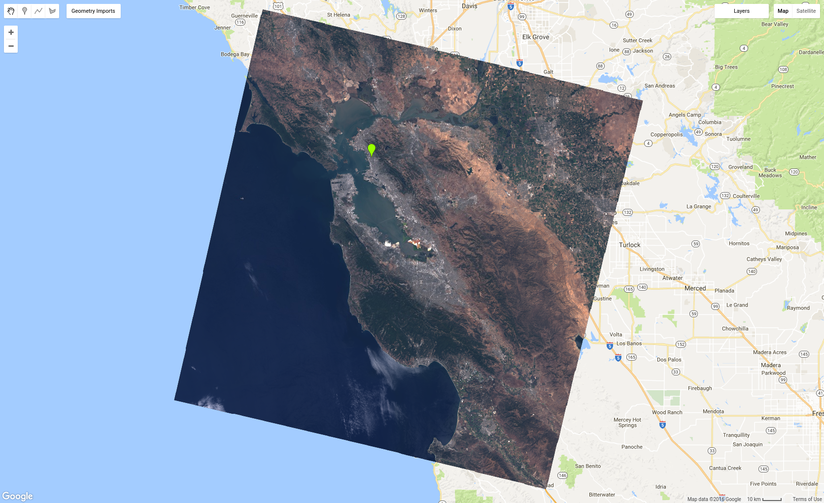
(scenein the previous example) to the map, the result is unsatisfactory:
Note that first, the map is centered on the image at zoom scale 9. Then the image is
displayed with an empty object ({}) for thevisParamsparameter
(see theMap.addLayer()docs for details). As a result, the image is
displayed with the default visualization: first three bands map to R, G, B, respectively,
and stretched to [0, 1] since the bands arefloatdata type. This means that
the coastal aerosol band ('B1') is rendered in red, the blue band ('B2') is rendered
in green, and the green band ('B3') is rendered in blue. To render the image as a
true-color composite, you need to tell Earth Engine to use the Landsat 8 bands 'B4', 'B3',
and 'B2' for R, G, and B, respectively. Specify which bands to use with thebandsproperty of thevisParamsobject. Learn more about
Landsat bands atthis
reference.
You also need to provideminandmaxvalues suitable for
displaying reflectance from typical Earth surface targets. Although lists can be used to
specify different values for each band, here it's sufficient to
specify0.3asmaxand use the default value of zero for theminparameter. Combining the visualization parameters into one object and
displaying:
The result should look something like Figure 5. Note that this code assigns the object
of visualization parameters to a variable for possible future use. As you'll soon
discover, that object will be useful when you visualize image collections!
Figure 5. Landsat 8 TOA reflectance image as a true-color composite,
stretched to [0, 0.3].
Try playing with visualizing different bands. Another favorite combination is 'B5', 'B4',
and 'B3' which is called a false-color composite. Some other interesting false-color
composites are describedhere.
Since Earth Engine is designed to do large-scale analyses, you are not limited to working
with just one scene. Now it's time to display a whole collection as an RGB composite!
Displaying image collections
Adding an image collection to a map is similar to adding an image to a map. For
example, using 2016 images in thel8collection and thevisParamsobject defined previously,
Note that now you can zoom out and see a continuous mosaic where Landsat imagery
is collected (i.e. over land). Also note that when you use theInspectortab and click on the image, you'll see a list of pixel values (or a chart) in thePixelssection and a list of image objects in theObjectssection of the inspector.
If you zoomed out enough, you probably noticed some clouds in the mosaic. When
you add anImageCollectionto the map, it is displayed as a recent-value
composite, meaning that only the most recent pixels are displayed (like callingmosaic()on the collection). That is why you can see discontinuities betweenpathswhich were acquired at
different times. It's also why many areas may appear cloudy. In the next page, learn how
to change the way the images are composited to get rid of those pesky clouds!
[[["Easy to understand","easyToUnderstand","thumb-up"],["Solved my problem","solvedMyProblem","thumb-up"],["Other","otherUp","thumb-up"]],[["Missing the information I need","missingTheInformationINeed","thumb-down"],["Too complicated / too many steps","tooComplicatedTooManySteps","thumb-down"],["Out of date","outOfDate","thumb-down"],["Samples / code issue","samplesCodeIssue","thumb-down"],["Other","otherDown","thumb-down"]],["Last updated 2023-10-06 UTC."],[],[]]

 ) and make a point in your area of
interest. Name the import
) and make a point in your area of
interest. Name the import  ), then expand the
list of
), then expand the
list of