Water Class Transition

The water transition layer captures changes between three classes of water occurrence (not water, seasonal water, and permanent water) along with two additional classes for ephemeral water (ephemeral permanent and ephemeral seasonal).

This section of the tutorial will:

1. add a map layer for visualizing water transition,
2. create a grouped reducer for summing the area of each transition class within a specified region-of-interest, and
3. create a chart that summarizes the area by transition class.

Basic Visualization

In the Asset List section of the script, add the following statement which creates a single band image object called transition :

 var 
  
 transition 
  
 = 
  
 gsw 
 . 
 select 
 ( 
 'transition' 
 ); 

The GSW images contain metadata on the transition class numbers and names, and a default palette for styling the transition classes. When the transition layer is added to the map, these visualization parameters will be used automatically.

At the bottom of the Map Layers section of your script, add the following statement which adds a new map layer that displays the transition classes:

 Map 
 . 
 setCenter 
 ( 
 105.26 
 , 
  
 11.2134 
 , 
  
 9 
 ); 
  
 // Mekong River Basin, SouthEast Asia 
 Map 
 . 
 addLayer 
 ({ 
  
 eeObject 
 : 
  
 transition 
 , 
  
 name 
 : 
  
 'Transition classes (1984-2015)' 
 , 
 }); 

When you run the script, the transition layer will be displayed.

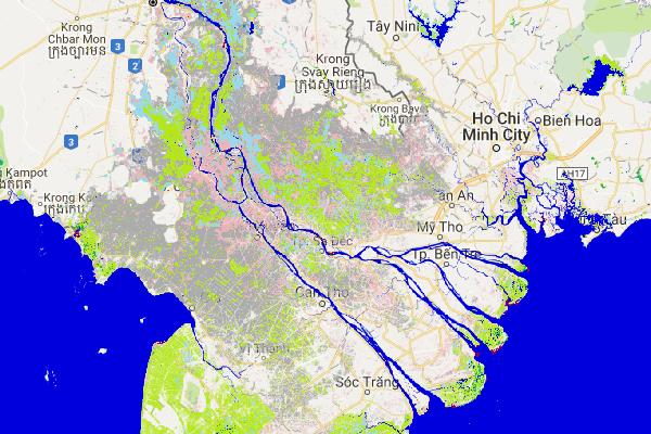
The map key for the transition classes is:

Summarizing Area by Transition Class

In this section we will once again use the geometry polygon tool to define a region-of-interest. If you want to analyze a new location, you will want to first select and delete the original polygon that you drew so that you don't get results from the combined areas. See the Geometry tools section of the Code Editor docs from information on how to modify geometries.

For this example we will draw a new polygon within the Mekong River delta.

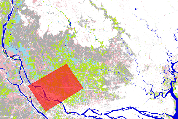
In order to calculate the area covered by parts of an image, we will add an additional band to the transition image object that identifies the size of each pixel in square meters using the ee.Image.pixelArea method.

 var 
  
 area_image_with_transition_class 
  
 = 
  
 ee 
 . 
 Image 
 . 
 pixelArea 
 (). 
 addBands 
 ( 
 transition 
 ); 

The resulting image object ( area_image_with_transition_class ) is a two band image where the first band contains the area information in units of square meters (produced by the ee.Image.pixelArea code> method), and the second band contains the transition class information.

We then summarize the class transitions within a region of interest ( roi ) using the ee.Image.reduceRegion method and a grouped reducer which acts to sum up the area within each transition class:

 var 
  
 reduction_results 
  
 = 
  
 area_image_with_transition_class 
 . 
 reduceRegion 
 ({ 
  
 reducer 
 : 
  
 ee 
 . 
 Reducer 
 . 
 sum 
 (). 
 group 
 ({ 
  
 groupField 
 : 
  
 1 
 , 
  
 groupName 
 : 
  
 'transition_class_value' 
 , 
  
 }), 
  
 geometry 
 : 
  
 roi 
 , 
  
 scale 
 : 
  
 30 
 , 
  
 bestEffort 
 : 
  
 true 
 , 
 }); 
 print 
 ( 
 'reduction_results' 
 , 
  
 reduction_results 
 ); 

The console tab output now displays the reduction_results . Note that you will need to expand the tree a few levels to see the area summary data.

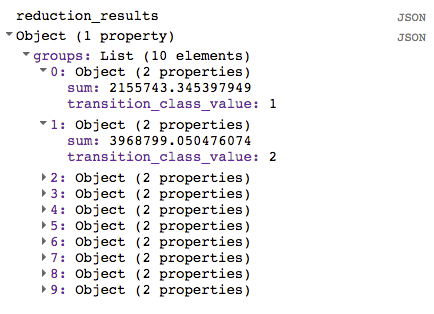
While the reduction_results object does contain information on the area covered by each transition class, it is not particularly easy to read. In the next section we will make it easier to view the results.

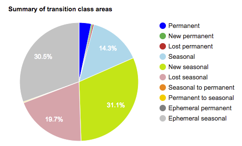
Creating a Summary Chart

In this section we will make a chart to better summarize the results. To get started, we first extract out the list of transition classes with areas as follows:

 var 
  
 roi_stats 
  
 = 
  
 ee 
 . 
 List 
 ( 
 reduction_results 
 . 
 get 
 ( 
 'groups' 
 )); 

The result of the grouped reducer ( reduction_results ) is a dictionary containing a list of dictionaries. There is one dictionary in the list for each transition class. These statements use the ee.Dictionary.get method to extract the grouped reducer results from that dictionary and casts the results to an ee.List data type, so we can access the individual dictionaries.

In order to make use of the charting functions of the Code Editor , we will build a FeatureCollection that contains the necessary information. To do this we first create two lookup dictionaries and two helper functions. The code that creates the lookup dictionaries can be placed at the top of the "Calculations" section as follows:

 ////////////////////////////////////////////////////////////// 
 // Calculations 
 ////////////////////////////////////////////////////////////// 
 // Create a dictionary for looking up names of transition classes. 
 var 
  
 lookup_names 
  
 = 
  
 ee 
 . 
 Dictionary 
 . 
 fromLists 
 ( 
  
 ee 
 . 
 List 
 ( 
 gsw 
 . 
 get 
 ( 
 'transition_class_values' 
 )). 
 map 
 ( 
 numToString 
 ), 
  
 gsw 
 . 
 get 
 ( 
 'transition_class_names' 
 ) 
 ); 
 // Create a dictionary for looking up colors of transition classes. 
 var 
  
 lookup_palette 
  
 = 
  
 ee 
 . 
 Dictionary 
 . 
 fromLists 
 ( 
  
 ee 
 . 
 List 
 ( 
 gsw 
 . 
 get 
 ( 
 'transition_class_values' 
 )). 
 map 
 ( 
 numToString 
 ), 
  
 gsw 
 . 
 get 
 ( 
 'transition_class_palette' 
 ) 
 ); 

The lookup_names dictionary associates transition class values with their names, while the lookup_palette dictionary associates the transition class values with color definitions.

The two helper functions can be placed in a new code section called "Helper functions".

Code Editor (JavaScript)

 ////////////////////////////////////////////////////////////// 
 // Helper functions 
 ////////////////////////////////////////////////////////////// 
 // Create a feature for a transition class that includes the area covered. 
 function 
  
 createFeature 
 ( 
 transition_class_stats 
 ) 
  
 { 
  
 transition_class_stats 
  
 = 
  
 ee 
 . 
 Dictionary 
 ( 
 transition_class_stats 
 ); 
  
 var 
  
 class_number 
  
 = 
  
 transition_class_stats 
 . 
 get 
 ( 
 'transition_class_value' 
 ); 
  
 var 
  
 result 
  
 = 
  
 { 
  
 transition_class_number 
 : 
  
 class_number 
 , 
  
 transition_class_name 
 : 
  
 lookup_names 
 . 
 get 
 ( 
 class_number 
 ), 
  
 transition_class_palette 
 : 
  
 lookup_palette 
 . 
 get 
 ( 
 class_number 
 ), 
  
 area_m2 
 : 
  
 transition_class_stats 
 . 
 get 
 ( 
 'sum' 
 ) 
  
 }; 
  
 return 
  
 ee 
 . 
 Feature 
 ( 
 null 
 , 
  
 result 
 ); 
  
 // Creates a feature without a geometry. 
 } 
 // Create a JSON dictionary that defines piechart colors based on the 
 // transition class palette. 
 // https://developers.google.com/chart/interactive/docs/gallery/piechart 
 function 
  
 createPieChartSliceDictionary 
 ( 
 fc 
 ) 
  
 { 
  
 return 
  
 ee 
 . 
 List 
 ( 
 fc 
 . 
 aggregate_array 
 ( 
 "transition_class_palette" 
 )) 
  
 . 
 map 
 ( 
 function 
 ( 
 p 
 ) 
  
 { 
  
 return 
  
 { 
 'color' 
 : 
  
 p 
 }; 
  
 }). 
 getInfo 
 (); 
 } 
 // Convert a number to a string. Used for constructing dictionary key lists 
 // from computed number objects. 
 function 
  
 numToString 
 ( 
 num 
 ) 
  
 { 
  
 return 
  
 ee 
 . 
 Number 
 ( 
 num 
 ). 
 format 
 (); 
 }